样样通吃的 Jev:从零构建并训练 Jev 式决策模型
Jev 风格决策模型与 Qwen 大语言模型在病理图像上的对比
构建一个受 Jev 启发的模型,将图像与答案选项进行比对。我们使用一个现有的病理图像—文本模型,并针对图像表示训练一个小的调整模块,称为 adapter。本教程展示如何构建和评估这一接口。
在相同的病理问题上,我们受 Jev 启发的模型击败了所测试的 Qwen 模型。在熟悉类别上,正确最终决策的比例约为 67.00% 对 43.00%;在新增类别上为 66.00–67.00% 对 40.00%。我们测试的具备图像能力的语言模型是 Qwen2.5-VL-3B-Instruct;我们并未对 Jev 本身进行基准测试。
针对熟悉组织训练的专用分类器在这方面表现更强。该线性分类器在 98.00% 的情况下选择正确,并在拒绝后 88.00% 的情况下作出正确的最终决策。其固定的输出头对新增类别没有输出。
起始的病理模型本身已经是一个很强的参照点。在额外的训练之前,它在新增类别上达到了 69.00% 的正确最终决策率。在拒绝之前,起始版本和训练后版本选择正确的比例均约为 77.00%。尝试更宽的 adapter 和更长的训练,也未能相对其匹配基线提升新增类别的召回率。
灵活的答案选项仍需要仔细评估。对于未提供正确答案的案例,adapter 仅拒绝了约 45.00%。所有后续测试结果都是探索性的,因为我们已经检查过测试集。整合后的 notebook 保留了这些实验与证据。
1. 动机:我为什么想构建这个
第1部分介绍了在给定答案中进行选择的 Jev 风格模型;第2部分在银行业务请求上测试了开源实现。这里我们将为图像构建一个这样的模型,并将其与具备图像能力的语言模型和经过训练的分类器进行比较。
我见过的大多数示例都使用文本。我在计算机视觉和医学影像方面的背景,包括乳腺成分成像和生成可分析的 DXA 图像,将我引向了病理学:向模型展示一张组织图像,并要求它选择匹配的描述。
提供的答案选项构成一个候选集,每个选项都是一个候选。“菜单”是一种非正式类比。分类器无需重新训练即可处理较少的熟悉选项,但支持一个新标签需要更新并训练其输出层。我们受 Jev 启发的模型可以接受新的书面描述,而无需进行进一步的特定任务训练。我们测试的是它能否正确识别该组织。
我们基于 Knowledge-Enhanced Pathology (KEEP) 构建受 Jev 启发的模型,这是一个经过训练以连接图像和文本的现有模型。我们保持该模型不变,并训练一个小型图像调整组件,称为适配器。我们将训练后的版本与未更改的初始模型 Qwen2.5-VL-3B-Instruct 以及传统分类器进行比较。Jev 启发了决策接口;Jev 本身并不属于该基准测试的一部分。
2. 该 notebook 展示了什么以及我们如何比较
我们使用 PathMNIST,这是一个通过 MedMNIST 分发的九类结直肠组织图像分类数据集。这九个类别分别是脂肪组织、背景、碎屑、淋巴细胞、黏液、平滑肌、正常结肠黏膜、癌相关间质和结直肠腺癌上皮。按照 MedMNIST 官方数据集元数据的记录,PathMNIST 以知识共享署名 4.0(CC BY 4.0)协议分发。图 1 由作者使用 PathMNIST 图像汇编而成,底层数据归属于 MedMNIST 以及 Kather 等人的源数据集。MedMNIST 除提供更小尺寸的变体外,还提供 224 像素版本。该数据集是研究与教育用途的资源;识别其组织标签并不能构成对患者的诊断。官方元数据,MedMNIST。
图 1。九个组织类别各取两个 PathMNIST 图像块,展示组织之间的差异以及同一类别内部的变异。我们固定图像不变,只改变模型可选择的标签。(图片由作者提供)
十八个组织图像块以三乘三的网格排列,每个类别给出两个示例:脂肪组织、背景、碎屑、淋巴细胞、黏液、平滑肌、正常结肠黏膜、癌相关间质和结直肠腺癌上皮。这些示例展示了类别之间的差异以及同一类别内部的变异。
我们的起点病理模型可处理图像和文本。这类模型被称为视觉语言模型(VLM)。大语言模型(LLM)生成语言;像 Qwen 这样具备图像能力的语言模型则同时符合这两种描述。这些标签彼此重叠,因此我用模型名称来区分各对比对象。我们的起点病理模型提供图像编码器和文本编码器。我们冻结这些编码器,并比较它们的数值表示,即嵌入。其作者描述的是知识增强的图像—文本预训练;我们不会从这一描述中推断 PathMNIST 概念或图像的缺失。该公开 checkpoint 采用 MIT 许可。模型卡,Zhou 等,Cancer Cell,2026。
我们的对比包含三个部分。第一,线性与非线性分类器使用与我们受 Jev 启发的模型相同的冻结 KEEP 图像向量。这样在比较不同拟合决策组件时,控制了表示这一变量。第二,我们实际从公开预训练 checkpoint 出发,微调了卷积神经网络 ConvNeXt V2 tiny 和视觉 Transformer EVA-02 base。CNN 通过卷积操作构建视觉表示;视觉 Transformer 则用注意力处理图像块。这些都是有代表性的强架构,但我们并不声称其中任一 checkpoint 是当前最佳的 PathMNIST 方法。它们不同的预训练、规模和预处理都应纳入解读。ConvNeXt V2 论文,EVA-02 论文。第三,Qwen2.5-VL-3B-Instruct 接收图像和书面答案选项,并生成一个选项字母或 NONE。这一对比考察的是在同一批问题上生成答案是否有帮助;它使用匹配的子集和保存的 KEEP 预测。
将图像与提供的答案描述进行比较。我们训练一个小型图像调整组件,称为适配器(adapter),同时保持起始模型不变。
起始病理模型(图中为“Unadapted KEEP”)
在没有我们额外训练的情况下进行相同的图像—描述比较。这是我们的训练前基线。
一个具备图像能力的语言模型,它读取图像和答案选项,然后写出选项字母或 NONE。
为熟悉的组织标签学习输出。它们可以在更少的这些标签中做选择,但要支持新增标签则需要进一步训练。
三条受 Jev 启发的线是同一模型的训练配方:所有选择、变化的选择,以及带有偏离起始模型惩罚的变化选择。图例中的 CE 表示交叉熵,即正确答案训练惩罚。我们测试的是我们的实现,而不是 Jev 本身。接受一个新描述并不保证能正确识别其组织。
为什么要自己构建模型?
我希望读者看到如何构建一个能在提供的描述中做选择的模型、训练它,并将其决策与语言模型和传统分类器进行比较。保存的图像特征使较小的实验便于复现;完整的图像模型训练是可选的。
为了公平比较,我们的任务特定训练只使用六个熟悉的组织类别。一个已经在全部九类上训练过的分类器会学到我们故意留出的答案。这是一个教学实验,并不是声称要击败当前最好的图像模型。
同一张图像,三组不同的候选集
取同一个标记为脂肪组织的图像块。在一个折中,脂肪组织是熟悉的;在另一个折中,它被排除在任务特定拟合之外。熟悉性描述的是某个特定的已拟合模型,而不是该组织的永久属性。
在脂肪组织为熟悉的折中,提供脂肪组织、正常结肠黏膜和基质
两种方法都能正确地将结果限定在现有目录内吗?
在排除脂肪组织的折中,提供脂肪组织、淋巴细胞和平滑肌
所提供的脂肪组织描述能否胜过熟悉的备选项?
对于同一个排除脂肪组织的模型,提供淋巴细胞和平滑肌
拒答策略会拒绝一个不可用的答案吗?
在三行中,该图像块都是相同的;第一行使用的拟合包含其类别,而后两行使用的拟合将其排除。被排除在教程拟合之外,并不意味着在 KEEP 预训练中不存在。省略一个已知组织答案也不能模拟所有可能的未知疾病。
原文较长,译文为节选;译文由英文原文机器翻译,术语按行业惯例统一,可在文末展开原文核对。
查看英文原文(A Jev of All Trades: Build and Train a Jev-style Decision Model From Scratch)
Jev-Style Decision Model vs Qwen LLM on Pathology Images
Build a Jev-inspired model that compares images with the answer options. We use an existing pathology image–text model and train a small adjustment to the image representation, called an adapter. The tutorial shows how to build and evaluate that interface.
Our Jev-inspired model beat the Qwen model we tested on the same pathology questions. Correct final decisions were about 67.00% versus 43.00% for familiar categories, and 66.00–67.00% versus 40.00% for added categories. The image-capable language model we tested was Qwen2.5-VL-3B-Instruct; we did not benchmark Jev itself.
A classifier trained for the familiar tissues was stronger there. The linear classifier chose correctly 98.00% of the time and made correct final decisions 88.00% of the time after rejection. Its fixed output head has no output for an added category.
The starting pathology model was already a strong reference point. Before our extra training, it reached 69.00% correct final decisions on added categories. Before rejection, the starting and trained versions chose correctly about 77.00% of the time. Trying wider adapters and longer training also failed to improve added-category recall over its matched baseline.
Flexible answer options still need careful evaluation. The adapter rejected only about 45.00% of cases with no correct answer offered. All follow-up test results are exploratory because we had already inspected the test set. The consolidated notebook preserves the experiments and evidence.
1. Motivation: why I wanted to build this
Part 1 introduced Jev-style models that choose among supplied answers; Part 2 tested open implementations on banking requests. Here we’ll build one for images and compare it with an image-capable language model and trained classifiers.
Most examples I had seen used text. My background in computer vision and medical imaging, including compositional breast imaging and generating analyzable DXA images, led me to pathology: show a model a tissue image and ask it to select the matching description.
The supplied answer options form a candidate set, and each option is a candidate. “Menu” is an informal analogy. A classifier can handle fewer familiar options without retraining, but supporting a new label requires updating and training its output layer. Our Jev-inspired model can accept a new written description without further task-specific training. Whether it recognizes that tissue correctly is what we test.
We build our Jev-inspired model from Knowledge-Enhanced Pathology (KEEP), an existing model trained to connect images and text. We leave that model unchanged and train a small image-adjustment component, called an adapter. We compare our trained version with the unchanged starting model, Qwen2.5-VL-3B-Instruct and conventional classifiers. Jev inspired the decision interface; Jev itself is not part of this benchmark.
2. What the notebook demonstrates and how we compare
We use PathMNIST, a nine-category colorectal tissue-image classification dataset distributed through MedMNIST. The categories are adipose, background, debris, lymphocytes, mucus, smooth muscle, normal colon mucosa, cancer-associated stroma and colorectal adenocarcinoma epithelium. PathMNIST is distributed under Creative Commons Attribution 4.0 (CC BY 4.0), as recorded in the official MedMNIST dataset metadata. Figure 1 is assembled by the author from PathMNIST images, with the underlying data credited to MedMNIST and the source dataset by Kather et al. MedMNIST supplies a 224-pixel version alongside smaller variants. The dataset is a research and educational resource; recognizing its tissue labels does not establish a patient diagnosis. Official metadata, MedMNIST.
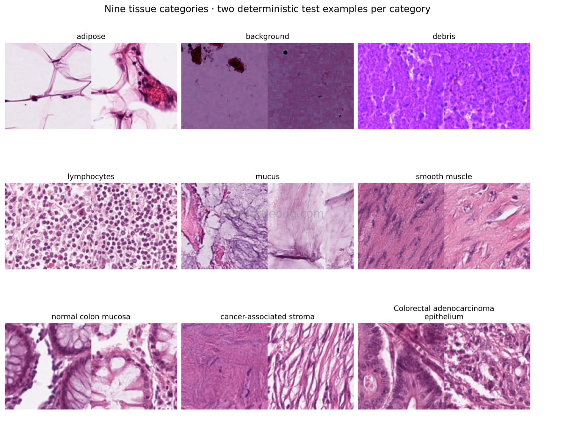
Figure 1. Two PathMNIST patches from each of nine tissue categories, showing differences between tissues and variation within each category. We keep an image fixed while changing which labels the model can choose. (Image by author)
Eighteen tissue-image patches arranged in a three-by-three grid, with two examples per category: adipose, background, debris, lymphocytes, mucus, smooth muscle, normal colon mucosa, cancer-associated stroma, and colorectal adenocarcinoma epithelium. The examples illustrate differences between categories and variation within each category.
Our starting pathology model works with images and text. Such a model is called a vision-language model (VLM). A large language model (LLM) generates language; an image-capable language model such as Qwen can fit both descriptions. These labels overlap, so I use the model names to distinguish the competitors. Our starting pathology model supplies image and text encoders. We freeze those encoders and compare their numerical representations, or embeddings. Its authors describe knowledge-enhanced image–text pretraining; we do not infer absence of PathMNIST concepts or images from that description. The public checkpoint is MIT licensed. Model card, Zhou et al., Cancer Cell, 2026.
Our comparison has three parts. First, linear and nonlinear classifiers use the same frozen KEEP image vectors as our Jev-inspired model. This controls the representation while comparing different fitted decision components. Second, we actually fine-tune a convolutional neural network, ConvNeXt V2 tiny, and a vision transformer, EVA-02 base, from public pretrained checkpoints. A CNN builds visual representations through convolutional operations; a vision transformer processes image patches with attention. These are strong representative architectures, without a claim that either checkpoint is the current best PathMNIST method. Their different pretraining, sizes and preprocessing belong in the interpretation. ConvNeXt V2 paper, EVA-02 paper. Third, Qwen2.5-VL-3B-Instruct receives the image and written answer options and generates an option letter or NONE. That comparison asks whether generating an answer helps on the same questions; it uses a matched subset and saved KEEP predictions.
Compares an image with the supplied answer descriptions. We train a small image-adjustment component, called an adapter, while leaving the starting model unchanged.
Starting pathology model (“Unadapted KEEP” in the figures)
Makes the same image–description comparisons without our extra training. This is our before-training baseline.
An image-capable language model that reads the image and answer options, then writes an option letter or NONE.
Learn outputs for the familiar tissue labels. They can choose among fewer of those labels, but supporting an added label requires further training.
The three Jev-inspired lines are training recipes for the same model: all choices, changing choices, and changing choices with a penalty for departing from the starting model. CE in the figure legends means cross-entropy, the correct-answer training penalty. We test our implementation, not Jev itself. Accepting a new description does not guarantee recognizing its tissue correctly.
Why build the model ourselves?
I want readers to see how to build a model that chooses among supplied descriptions, train it, and compare its decisions with a language model and conventional classifiers. Saved image features keep the smaller experiments practical to reproduce; complete image-model training is optional.
For a fair comparison, our task-specific training uses only the six familiar tissue categories. A classifier already trained on all nine would have learned the answers we deliberately hold out. This is a teaching experiment, not a claim to beat the best available image model.
One image, three different candidate sets
Take the same patch labeled adipose. In one fold adipose is familiar; in another it is excluded from task-specific fitting. Familiarity describes a particular fitted model, not a permanent property of the tissue.
In a fold where adipose is familiar, offer adipose, normal colon mucosa and stroma
Can both methods restrict the existing catalog correctly?
In the fold excluding adipose, offer adipose, lymphocytes and smooth muscle
Can the supplied adipose description win against familiar alternatives?
For that same excluded-adipose model, offer lymphocytes and smooth muscle
Does the rejection policy decline an unavailable answer?
The patch is the same in all three rows; the first row uses a fit that includes its category, and the next two use the fit that excludes it. Excluded from tutorial fitting does not mean absent from KEEP pretraining. Omitting a known tissue answer also does not simulate every possible unknown disease.
The preserved development cohort has 900 images drawn from the official validation collection. Each tissue contributes 80 training and 20 validation examples. Of the twenty validation examples, eight select hyperparameters and checkpoints, six fit temperature, and six fit the rejection threshold. Only familiar categories participate in those fitting roles. Each of three outer category folds excludes three categories; training repeats use seeds 7, 17 and 27. Inner selection temporarily excludes two of the six familiar categories to evaluate transfer without consulting the outer-excluded categories.
The official 7,180-image test collection is reused for final evaluation. It has already appeared in tutorial development. This is an exploratory, prespecified follow-up, not an untouched confirmation set. Source-image IDs support separation of these roles; they do not establish patient-level independence or rule out foundation-model pretraining overlap. The official metadata describes a different clinical center for the test images. Dataset provenance.
The notebook protocol cell freezes the wording bank, partitions, candidate sets, tolerances and comparison settings. Three templates train, one selects, and two evaluate new wording. The two historical templates remain reference conditions.
3. Comparing our Jev-inspired model, Qwen and classifiers
These earlier experiments measure class-macro recall: each tissue’s correct-choice rate gets equal weight, before any answers are declined. The later Qwen comparison uses 270 matched test patches and also measures decisions after rejection, so compare percentages within each evaluation. Repeated questions about one image are not independent samples.
Familiar tissues: classifiers are strong
A classifier can choose among fewer familiar labels without retraining: ignore the outputs outside the supplied candidate set. On these questions, the classifiers reached 96.22–97.96% average recall, versus 84.59% for our Jev-inspired model trained with all six choices. The linear and nonlinear classifiers share our model’s image features; the complete convolutional-network and transformer classifiers also change the image processing.
Our model’s answers stayed unchanged across 3,888 choice-order checks and 72 checks that renamed internal answer IDs. Changing the descriptions did change the scores: the text tells the model what each answer means.
Added tissues: descriptions allow new answer options
A fixed-label classifier needs its output layer updated and trained to support an added category. Our Jev-inspired model can evaluate its written description without further training. Added-category recall was 70.97% for the starting pathology model and 71.81–72.02% across our three training recipes. These categories were excluded from our training, but may have appeared in the starting model’s earlier training.
More choices made recognition harder. For the changing-choices recipe with preservation, added-category recall fell from 90.04% with two options to 58.52% with nine (Figure 2). Accepting a new description does not guarantee recognizing it correctly.
Figure 2. Recognition declines as the number of choices grows, with familiar and added tissue categories shown separately. Each tissue receives equal weight. Points summarize repeated questions about the same test images, not independent patient cohorts. (Image by author)
Class-macro recall across candidate sets containing two to nine answers. Fixed classifiers perform best on familiar categories within their supported label sets. For added categories, KEEP and the trained adapters show similar declines as more alternatives compete. Categories receive equal weight; repeated evaluations reuse the same test images.
We reuse one fitted Jev-inspired model across these questions. For nine categories there are 502 subsets containing at least two choices: 255 contain a given image's correct answer and 247 omit it. Because each raw image–description score is computed independently of the other choices, we can save nine scores per image and derive all those candidate set results without repeatedly encoding the image.
Does practicing with changing candidate sets improve recognition?
This was the original adapter-training question. We compare four versions: unadapted KEEP; an adapter trained with all six familiar choices; an adapter trained on sampled candidate sets of two through six choices; and the sampled version with an extra penalty for moving away from KEEP's original shares. We call the last version sample-preserve in the figures. Section 4 works through that penalty.
All three trained KEEP adapter variants use matched image presentations and optimizer budgets, and the same training wording bank. With familiar truth competing against a mixture of familiar and added alternatives, all-six-choice training reached 76.28%, sampled cross-entropy reached 76.22%, and sample-preserve reached 75.98%. Unadapted KEEP reached 70.16%. Training the adapter helped in this comparison, but sampling the candidate sets did not improve on the simpler full-set recipe.
Figure 3. Familiar tissue recognition when choosing among familiar labels and when added labels also compete. Compare methods within the same candidate-set condition. Fixed classifiers are evaluated only where their output heads support every offered category. (Image by author)
Class-macro recall for familiar tissue categories under familiar-only and mixed candidate sets. Fixed classifiers lead where all offered categories are supported by their output heads. Training KEEP adapters with changing choices did not improve familiar mixed-set recall over all-six-choice training.
The paired comparison keeps each image's results together when estimating uncertainty. Sampled cross-entropy was 0.07 percentage points below all-six-choice training, with a 95.00% interval of −0.11 to −0.03. Sample-preserve was 0.30 points below, with an interval of −0.35 to −0.25. These are small differences, but they do not support the improvement we set out to test.
Added-category recall was slightly higher: +0.15 and +0.21 points, respectively, with intervals above zero. Both recipes met 17 of the other 18 size and wording conditions, but failed the primary familiar mixed-candidate set improvement condition. These intervals describe uncertainty conditional on this dataset and design. They do not establish patient-level independence or guarantee that all conditions hold together.
Figure 4. Recall changes relative to all-six-choice training, with paired 95% bootstrap intervals. Positive differences favor the sampled-choice recipe. Small gains for added categories did not offset the failed primary improvement criterion for familiar categories. Resampling keeps repeated records from each source image together. (Image by author)
Paired recall differences for sampled-choice training, with and without a preservation penalty, relative to all-six-choice training. Both recipes missed the primary improvement criterion for familiar categories competing with added alternatives. Intervals keep repeated observations from each source image together and do not establish patient-level independence.
Wording gives us another reason to be cautious. On the two descriptions reserved for evaluation, sample-preserve's familiar mixed-candidate set recall was 84.43% versus 69.57%; added-category recall was 77.45% versus 66.97%. The tissue identities stayed the same, but the phrasing changed. Two templates are only a small language check, and this spread makes it difficult to argue that wording is an unimportant detail.
Figure 5. Two description templates excluded from training and selection produce different recognition results. The tissue identities stay the same, but changing their descriptions changes performance. Two templates provide a limited wording check, not evidence of broad language robustness. (Image by author)
Recall changes substantially between two description templates excluded from training and selection. For the preservation recipe, familiar-category recall was 84.43% versus 69.57%, and added-category recall was 77.45% versus 66.97%. The tissue identities stayed the same, showing that wording can materially affect recognition.
What if the right answer is missing, or the score looks too confident?
Return to the adipose image, but offer only lymphocytes and smooth muscle. Softmax will still divide all its share between those two choices. One of them must receive the larger share even though neither is correct. A large share therefore cannot, by itself, tell us that the candidate set contains a valid answer.
We fit a separate rejection threshold using familiar validation examples, choosing a threshold that retained at least 95.00% of answer-present examples there. On the held-out evaluation candidate sets, sample-preserve retained 82.72% of answer-present cases and rejected 44.85% of answer-absent cases. Put another way, it still accepted 55.15% of candidate sets missing the answer. The fitting target did not carry over as a guarantee.
Figure 6. Rejection trades how often the model answers against the errors it makes and the missing answers it detects. Retaining an example does not mean answering it correctly. These experiments remove known tissue labels from the candidate set; they do not establish detection of unknown diseases. (Image by author)
Rejection trades answer coverage against errors and detection of missing answers. The preservation recipe retained 82.72% of answer-present cases and rejected 44.85% of answer-absent cases. Accepting a case does not mean answering it correctly. These experiments omit known tissue labels; they do not establish detection of unknown diseases.
We also tried temperature scaling, which adjusts how concentrated the shares are without changing the highest-scoring answer. A calibrated 80.00% confidence would mean that, over comparable predictions receiving that confidence, about 80.00% are correct. Our fitted temperature did not improve that agreement on the transferred evaluation conditions.
For sample-preserve, familiar negative log-likelihood (NLL) rose from 0.56 to 78.12, and added-category NLL from 0.68 to 165.03. NLL penalizes assigning little share to the correct answer, so lower is better. Expected calibration error (ECE), which compares confidence and observed accuracy within bins, also worsened: 3.15% to 19.18% for familiar truth and 5.05% to 23.86% for added truth. The very large NLL values show why we should inspect more than the selected answer or a single calibration summary. Section 4 explains how the same ranking can produce very different shares.
We independently recomputed these values from the saved logits and reproduced both increases. The nine fitted temperatures ranged from approximately 0.000912 to 0.270, with two reaching the allowed lower bound, exp(−7). Each fit used only 36 familiar-category calibration images under the selection wording. Very small temperatures amplify score differences, so incorrect predictions can assign effectively zero probability to the true answer and incur enormous NLL without changing which answer wins. This is a pathological calibration-transfer result, not evidence of useful calibration.
Figure 7. Reliability before and after fitting a temperature on a separate familiar-category partition. Agreement between reported confidence and observed correctness is the goal. Here, the adjustment worsened measured NLL and ECE on evaluation candidate sets; fitting a calibration parameter does not establish that confidence transfers reliably. (Image by author)
Reliability curves for familiar and added tissue categories. The diagonal represents agreement between confidence and observed accuracy. Temperature scaling, fitted on a separate familiar-category partition, worsened negative log-likelihood and expected calibration error on the evaluation candidate sets. The adjustment preserves answer rankings but does not guarantee reliable confidence under changed conditions.
Both the KEEP adapter and classifier helpers can return the same structured fields: candidate IDs, scores, shares, chosen ID, and whether the answer was rejected. A rejected answer has a null selected ID. This makes the result straightforward to integrate into software, but the format itself cannot tell us whether the decision was correct.
What does the flexibility cost?
The complete-model comparison includes nine fold/seed fits for each architecture, each selected from two learning-rate trials. Their fresh heads learn only the six familiar categories. These results complement the shared-KEEP-feature experiment; different pretraining and image encoders prevent attributing every difference to the output interface alone.
For a single image with candidate text already cached, sample-preserve's median image-to-decision time was 64.54–71.00 ms across candidate sets of two through six choices. ConvNeXt took 10.04–10.07 ms and EVA-02 23.18–23.46 ms over supported sizes. Our Jev-inspired model's 95th-percentile times were 67.03 ms at two choices and 73.33 ms at six. These measurements used the same Tesla T4, float32 precision, twenty warmups and one hundred synchronized repeats.
Figure 8. Measured inference time for one image with candidate text cached. Timing includes image preprocessing, encoding, and the decision step, but excludes new-description encoding and cold setup. Fixed classifiers cannot support nine choices because each fitted head has six outputs. These measurements show no speed advantage for the KEEP adapter on this hardware and workload. (Image by author)
Batch-one inference timing on a Tesla T4, including image preprocessing, encoding, and the decision step, with candidate text cached. The KEEP adapter took approximately 65–71 milliseconds, compared with 10 milliseconds for ConvNeXt and 23 milliseconds for EVA-02 over supported candidate sets. Measurements exclude new-description encoding and cold setup.
Peak allocated memory in these paths was about 1.69 GB for sample-preserve, 152.00 MB for ConvNeXt and 375.00 MB for EVA-02. The run records 68 measured rows and eight unsupported conditions. We have no measured speed or memory advantage for our Jev-inspired model here. Dollar cost would additionally depend on the service, billing arrangement and workload; these timings alone do not establish a universal price.
What the notebook covers
The table keeps track of all fourteen questions. Each row has an implementation and saved evidence in the notebook. Coverage means we ran and examined the experiment, including where the result was unfavorable.
What the notebook demonstrates
Scores and recall computed for held-out categories; fixed classifiers report unsupported candidate sets.
Added truth versus distractors
Recall measured by composition and size; declines at larger candidate sets.
72 checks; ID rename gap 0; description reassignment changes scores.
Reuse across candidate sets
One fitted Jev-inspired model evaluated across 502 candidate sets per image.
Both sampled recipes miss the primary improvement criterion.
Two templates differ substantially; no broad robustness claim.
Familiar subset classifiers
All four classifier systems evaluated on matched supported candidate sets.
3,888 direct checks; zero gaps/flips.
Paired comparisons on the same images; sampled recipes do not improve familiar mixed-candidate set recall.
KEEP adapter and fixed-classifier examples saved with explicit rejection field.
Missing-answer rejection
82.72% present retention; 44.85% absent rejection for sample-preserve.
Temperature transfer worsens NLL and ECE in these data.
18 complete-model fits, with familiar-only training and separate selection.
Measured inference time and memory; unsupported conditions recorded separately.
Historical reference: what the earlier run actually measured
The preserved earlier run keep-tutorial-run-20261016T045308987029Z used the previous two-template protocol and full-set recipe. Its balanced accuracies averaged seeds within category folds, then averaged the three folds:
Familiar tissue, six choices
Familiar tissue, nine choices
Excluded tissue, nine choices
Earlier trained Jev-inspired model
These historical values are retained for context and are not substituted for the rotating-candidate set results above.
Follow-up: did a wider adapter or longer fit help?
The original Jev-inspired model used a 64-unit adapter and a short training budget. To examine that constraint, I reused the audited KEEP image features and cached text embeddings on a Colab Tesla T4. The predeclared development search crossed widths 32, 64 and 128 with epoch caps 20 and 40, keeping the sampled-set preservation recipe and each fold’s baseline-selected preservation weight fixed. Three inner development category splits selected settings by mean harmonic macro recall, then loss, narrower width and shorter cap. Three seeds refit each selected setting. The test set played no part in selection; because its results had already been inspected, this follow-up is exploratory rather than independent confirmation.
Development selection score
The development settings were close: all six mean selection scores round to 0.91. The notebook retains the small differences used for selection. The fold selections were mixed, so this search does not show that simply increasing capacity or duration consistently helps.
Figure 9. Mean harmonic recall from the development-only search over adapter width and training duration. Each outer fold selected its own width and epoch cap using full-precision scores; displayed values are rounded. The test set was not used for selection. (Image by author)
Development-only search comparing six adapter width and training-duration settings across three outer category folds. Selection uses harmonic mean recall for familiar and temporarily excluded categories. Each fold selects its own configuration using full-precision scores; displayed values are rounded. The test set was not used to select these settings.
On the exploratory test follow-up, added-category macro recall was 71.04% for the selected settings and 71.38% for the matched sampled-preserve baseline, a difference of −0.34 percentage points. Familiar-category recall was 76.47% versus 76.19% (+0.27 points). These small opposing differences do not support a general accuracy advantage for our Jev-inspired model or for a wider/longer adapter.
Cancer-associated stroma
Colorectal adenocarcinoma epithelium
The candidate-set-size pattern was similar for both methods:
Figure 10. Familiar- and added-category recall across candidate-set sizes for the baseline and development-selected adapter settings. The two methods track closely. Results average over folds, seeds, and evaluation wordings; repeated questions reuse the same source images. (Image by author)
Exploratory test recall across candidate-set sizes for the baseline adapter and the settings selected by the width and training-duration search. The curves track closely, with no improvement in overall added-category recall from the selected settings. Results average over folds, seeds, and evaluation wordings.
The saved timings cover GPU fitting and scoring cached features only. Development fitting took 54.39 seconds across search fits, selected refits 8.79 seconds, and cached-feature test scoring 0.53 seconds across 36 timing rows. These timings exclude data acquisition, encoder work, archive transfer and notebook startup. They are not end-to-end reproduction times.
Did our Jev-inspired model beat the LLM comparator?
I also compared the trained Jev-inspired model with Qwen2.5-VL-3B-Instruct, a general-purpose vision-language model. Qwen receives the original 224-pixel image, the candidate descriptions and a request to return one option letter or NONE. Our Jev-inspired model uses the frozen KEEP image and text encoders plus its trained adapter to score those same supplied descriptions. This is one named model comparison; it is not a comparison with every LLM and it does not run Jev itself.
We chose Qwen2.5-VL-3B-Instruct as a public, image-capable generative comparator practical on a single Colab Tesla T4. The 18-image development pilot verified execution and estimated runtime; model and prompt choices were not selected using recognition accuracy. This resource-bounded comparison does not establish performance against the strongest available vision-language model or against LLMs generally.
The comparison uses the same 270 previously inspected test images for every method: 30 images from each tissue category. The paired baseline set includes unadapted KEEP, three trained KEEP adapters, and the linear and nonlinear KEEP-feature heads. ConvNeXt and EVA-02 remain in the earlier results; their scores were not part of this exact saved-score protocol, so I did not add an unmatched number to this table. Each image appears with three or six answer options, two held-out descriptions, and one of three conditions. The true answer is familiar to the fitted model, added as a category excluded from its task-specific fitting, or absent. The 3,240 Qwen requests use one frozen prompt and model revision. The 18-image validation pilot checked execution and set the sample count from runtime only. No test result selected a model or prompt. Since this test set had already been inspected, every number here is exploratory, not independent confirmation.
Familiar: correct decisions / correct choices
Added category: correct decisions / correct choices
Reject when answer is absent
Unadapted KEEP, description scoring
Our KEEP adapter, all-six-choice training
Our KEEP adapter, sampled-choice training
Our KEEP adapter, sampled-choice training with preservation
Linear classifier on KEEP features
Unsupported: its fixed head has no added-category output
Nonlinear classifier on KEEP features
Unsupported: its fixed head has no added-category output
“Correct choices” asks whether the selected category matches the tissue label, before rejection. “Correct decisions” also counts the fitted rejection rule: a supplied answer rejected by the model is not a correct decision, and an absent answer is correct only when the model rejects. Qwen returned an offered option for all 3,240 requests, including every answer-absent request. The KEEP models use rejection thresholds fit on their designated familiar-only validation examples. Classifier heads can score the familiar choices, but cannot score an added category they were never fitted to represent.
Yes: our Jev-inspired model beat Qwen2.5-VL-3B on this matched comparison. For added categories, the three training recipes made correct final decisions on 66.23–66.57% of cases, compared with 40.09% for Qwen. Unadapted KEEP reached 68.80%, so the trained adapter did not improve this final-decision measure. Before rejection, added-category correct choices were almost identical: 77.04% for unadapted KEEP and 77.10–77.22% for the adapters. The larger difference after rejection reflects their decision policies as well as recognition. Category results vary: Qwen reached 99.00–100.00% correct decisions on normal colon mucosa and colorectal adenocarcinoma in this sample, and 0.00–8.00% on adipose, debris and background. KEEP is pretrained specifically for pathology, while Qwen is general-purpose; this comparison combines differences in pretraining, representation and decision interface. These results support a comparison with this named Qwen model, prompt and task on 270 selected patches. They do not establish a general advantage over LLMs or a benefit caused by adding our adapter.
For familiar categories, the linear KEEP-feature classifier chose the right offered answer 98.00% of the time. Its final decision rate was lower, 88.00%, because it sometimes rejected. The trained Jev-inspired models made correct final decisions on about 67.00%, and Qwen on 43.00%. Familiar classification is already a strong use case for the fixed output head.
When the correct answer was absent, Qwen rejected none of these cases. Our Jev-inspired model rejected about 45.00%. The linear and nonlinear classifiers rejected 94.00% and 91.00% on these familiar-only choices under their saved thresholds. These are task-specific results; they do not establish general open-set detection or reliability.
Figure 11. Correct final decisions on the same exploratory test images and answer options, including each method’s rejection policy. Fixed classifiers are marked unsupported when the correct category has no output. Scores average equally over categories, wordings, candidate-set sizes, and saved baseline seeds. This comparison evaluates the named models, not Jev itself. (Image by author)
Matched exploratory comparison on 270 PathMNIST images. KEEP adapters outperformed Qwen2.5-VL-3B on familiar and added-category decisions, while fixed classifiers led on supported familiar categories. Unadapted KEEP had the highest added-category final-decision rate among the KEEP methods. Results include rejection behavior and reuse a previously inspected test set.
Figure 12. Correct final decisions with three and six answer options on the same exploratory test subset. More options generally lowered correct decisions when the answer was present. Qwen rejected none of the answer-absent cases at either size. Results include each method’s decision policy. (Image by author)
Candidate-set-size results from the matched exploratory comparison on 270 PathMNIST images. Increasing from three to six options generally lowered correct final decisions when the answer was present. Qwen rejected none of the answer-absent cases at either size. Fixed classifiers are evaluated only where their outputs support the supplied choices.
Figure 13. Added-category correct final decisions by tissue, showing variation hidden by the overall average. Categories were excluded from each fitted KEEP model’s task-specific training; this does not establish that their concepts were absent from pretraining. Results average across candidate-set sizes, wordings, and saved baseline seeds. (Image by author)
Added-category decision rates from the matched exploratory comparison, averaged across candidate-set sizes, description wordings, and saved baseline seeds. Performance varies substantially by tissue category. Categories were excluded from each fitted model’s task-specific training, but may have appeared in pretraining. Results include rejection behavior and reuse a previously inspected test set.
Qwen’s median time from an in-memory RGB image to a decoded answer was 0.19 seconds; its 95th-percentile time was 0.20 seconds across these requests on the Colab T4. This includes image processing and model generation, but excludes image-source reads and model setup. The earlier KEEP timing measures cached-feature scoring and cannot support a direct speed ratio. Model setup, weights, prompts, request records and hashes are saved with the notebook results. The test-set comparison remains exploratory because of prior inspection.
4. Inside the notebook: build it and adapt it
The single notebook has a default path using the audited frozen KEEP vectors. That path needs no tissue dataset download, model-account token or paid model API. New descriptions need frozen text encoding unless their embeddings are already cached. New images need image encoding. Optional complete-image-model reproduction additionally needs the native image cohort and public CNN/ViT initializations. Cached KEEP vectors cannot replace pixels for that experiment.
Start with the image–description score
A vector is a list of numbers. Its length is the square root of the sum of its squared entries. For [3,4], the length is sqrt(9+16)=5; normalization gives [0.60,0.80]. A dot product multiplies matching entries and adds them: [0.60,0.80]·[0,1]=0.80. The actual image and text representations have 768 entries.
The adapter compresses an image vector from 768 to 64 entries, applies GELU, and expands back to 768. Let that proposed update be r, and let x and t be the frozen image and normalized text vectors:
δ = 0.05 r / max(1, ‖r‖)
u = normalize(x + δ)
score(x,t) = a(u · t)
In plain English: KEEP gives us a numerical description of the image. The adapter proposes a small change to that description. We limit the size of the change, add it to the original, and compare the result with each tissue description.
x is the frozen image vector, a list of 768 numbers. t is the text vector for one candidate, scaled to length one.
r is the change proposed by the adapter. δ, the Greek letter delta, is the change we actually allow. The bars in ‖r‖ mean its length.
max(1, ‖r‖) means use whichever is larger: one or that length. Dividing by this number prevents a large proposed change from growing without limit. Multiplying by 0.05 sets the maximum update length.
u is the adjusted image vector, rescaled to length one. The dot in u · t means multiply matching entries and add their products. a is KEEP's fixed multiplier, which turns that similarity into a raw score, also called a logit.
For example, if the proposed change has length four, we divide it by four and multiply by 0.05. Its final length is 0.05. If its original length is 0.40, the denominator is one and its final length is 0.02. These are illustrative lengths, not measured predictions. Limiting how far the vector moves does not guarantee that its answers remain correct.
raw = self.up(F.gelu(self.down(x)))delta = self.alpha * raw / raw.norm(dim=-1, keepdim=True).clamp_min(1.)scores = LOGIT_SCALE * (F.normalize(x + delta, dim=-1) @ F.normalize(text, dim=-1).T)
Sample a candidate set and move the target with it
For each training image, sample a candidate set size uniformly from two through six, include its true category, sample distractors without replacement, then shuffle. Inner training uses two through four because only four categories are familiar there.
size = rng.integers(2, len(familiar_ids) + 1)others = [c for c in familiar_ids if c != true_id]candidate_options = rng.permutation([true_id, *rng.choice(others, size - 1, replace=False)])target_position = int(np.flatnonzero(candidate_options == true_id)[0])
If the true tissue is lymphocytes and the candidate set is [smooth muscle, lymphocytes, adipose], its target position is one in Python. Reordering to [adipose, smooth muscle, lymphocytes] moves that target to two. Retaining the old position would teach the wrong tissue. The actual implementation supports different candidate set lengths within a batch and excludes padded positions from the loss. See sample_training_menu in notebook menu_training.
Work through cross-entropy
Suppose the true tissue is lymphocytes and our candidate set is [smooth muscle, lymphocytes, adipose]. We will use illustrative logits [0.20,1.50,−0.30] and follow them all the way to the training penalty. These are example numbers, not a saved model prediction.
First, turn the scores into positive weights. The exponential function, written exp(s) or eˢ, raises the number e (about 2.72) to the score. A calculator's eˣ button does this. Even a negative score becomes a positive weight:
Next, divide each weight by the total. The weights sum to about 6.44. Smooth muscle receives 1.22 / 6.44 ≈ 0.19; lymphocytes receives 4.48 / 6.44 ≈ 0.70; and adipose receives 0.74 / 6.44 ≈ 0.11. This operation is softmax. We calculate with unrounded values and display two decimal places. The shares add to one; the correct answer’s unrounded share corresponds to 69.55%.
Finally, turn the correct answer's share into a penalty:
In plain English: Find the share assigned to the correct answer, take its natural logarithm (the ln button), and change the sign. CE means cross-entropy, the penalty we ask training to reduce.
A correct-answer share of 0.90 gives a small penalty, about 0.11. A share of 0.10 gives a larger penalty, about 2.30. Our example lies between them at 0.36. Training can reduce this penalty by increasing the correct answer's score relative to its alternatives. A 69.55% share is not yet a validated 69.55% chance of being right.
PyTorch performs these steps stably from the logits with F.cross_entropy(scores, target_position). We supply position one for lymphocytes in this candidate set, not its dataset category ID.
Add a preservation penalty
The training objective is:
L = CE + λ KL(pKEEP ‖ padapter)
KL(p ‖ q) = Σ pi ln(pi/qi)
In plain English: Train the adapter to select the correct tissue, while charging an extra penalty when its shares move away from KEEP's original shares on the same candidate set.
L is the total training penalty. CE is the correct-answer penalty we just calculated.
p is KEEP's list of shares and q is the adapter's list. The small i selects one candidate from those lists.
Σ, the capital Greek sigma, means add the following quantity over every candidate. For each candidate, divide its KEEP share by its adapter share, take the natural logarithm, and multiply by its KEEP share.
KL names this measure of disagreement between the two distributions. It is zero when the shares agree. λ, pronounced lambda, controls how much that disagreement contributes to training. Zero turns the extra penalty off.
For a two-choice example, let KEEP give shares p=[0.70,0.30] and the adapter give q=[0.60,0.40]. The first contribution is 0.70 × ln(0.70/0.60) ≈ 0.11; the second is 0.30 × ln(0.30/0.40) ≈ −0.09. Their sum is about 0.02. Individual contributions can be negative even though the total KL is nonnegative.
If the first choice is correct, cross-entropy is −ln(0.60) ≈ 0.51. At λ=0.10, the complete loss is 0.51 + 0.10 × 0.02 ≈ 0.51. These illustrative numbers show how the penalties combine; they do not establish that the extra term preserves recognition of excluded tissues.
with torch.no_grad(): teacher_probs = keep_scores.softmax(-1).detach()ce = F.cross_entropy(adapter_scores, targets)kl = F.kl_div(adapter_scores.log_softmax(-1), teacher_probs, reduction='batchmean')loss = ce + preservation_lambda * kl
The teacher is detached: gradients update the adapter, not KEEP. We sample one of the three training templates per update. All-six-choice CE uses that same wording policy so the objective comparison does not also change the bank of training text.
Inner selection considers recall S on four temporarily familiar categories and U on two temporarily added categories, with all six descriptions competing. It uses their harmonic mean H=2SU/(S+U), defined as zero if both recalls are zero. In plain English, this selection score rewards doing well on both groups. Multiply their recalls together, double the result, and divide by their sum. With S=0.90 and U=0.10, we get 2 × 0.90 × 0.10 / (0.90 + 0.10) = 0.18. Their ordinary average would be 0.50, which hides more of the poor added-category result. Selected epochs determine a common final adapter training budget. A selected preservation weight of zero or an epoch budget of zero remains an allowed result.
Build and train the CNN and ViT
The CNN starts from timm/convnextv2_tiny.fcmae_ft_in22k_in1k, revision b1dd46230e80bf4cc3fa0c3c905db2c3ec53a817. The transformer starts from timm/eva02_base_patch14_224.mim_in22k, revision 0ecfe3fab2be96198054b55157bd448097ba1828. Their cards describe distinct pretraining and preprocessing. The CNN weights carry CC-BY-NC-4.0 terms; the EVA-02 weights are MIT licensed. CNN card, ViT card.
For each outer fold, create a new six-output head and optimize it together with the pretrained backbone. The pinned checkpoint initializes visual knowledge; the new head learns the six familiar tissue identities. Use the checkpoint's resize/crop, normalization and interpolation settings; training also applies independent horizontal and vertical flips. This schematic shows the component setup; notebook classifier_benchmarks contains public-file resolution, exact revisions, initialization and resumable fitting.
model = timm.create_model(f'hf-hub:{repo}@{revision}', pretrained=True, num_classes=6)data_config = resolve_model_data_config(model)evaluate_transform = create_transform(**data_config, is_training=False)optimizer = torch.optim.AdamW(model.parameters(), lr=learning_rate, weight_decay=1e-4)
Both architectures use batch sixteen, float32 and at most twenty epochs per learning-rate candidate. The CNN searches 1.00e-4 and 1.00e-3; the ViT searches 1.00e-5 and 1.00e-4. Every epoch sees each permitted familiar training image once. Selection uses the eight designated validation images per familiar category, ranking macro recall, then cross-entropy, then earlier epochs; learning-rate ties prefer the lower rate. These are tutorial tuning budgets, not reproductions of published benchmark recipes. Different batch sizes mean the image models and small heads have different optimizer-update counts, which the run records.
The full grid is expensive: two rates, twenty epochs, three folds and three seeds for each architecture. The audited run records its memory and scoped runtime measurements in the notebook. The default reader path embeds those saved results; fresh image-model training is explicitly optional. Each finished epoch saves optimizer state, random-generator state, provenance and selected weights, so resuming does not require another image acquisition or KEEP encoding pass.
We have already turned logits into shares. Temperature scaling repeats that calculation after dividing every score by one positive number, T:
sharei = exp(scorei / T) / Σj exp(scorej / T)
In plain English: Divide each raw score by the temperature, turn the divided scores into positive weights, and divide each weight by their total. The small i identifies the candidate whose share we want; j runs through all candidates when calculating that total.
With two illustrative scores [2, 0] and T=1, the shares are about [0.88, 0.12]. At T=2, we first divide the scores to get [1, 0], giving shares [0.73, 0.27]. At T=0.50, the divided scores are [4, 0] and the shares become [0.98, 0.02]. The first choice wins every time, but its apparent confidence changes considerably.
We fit T using only the designated familiar calibration examples. Increasing it makes shares flatter; decreasing it makes them sharper. Because division by a positive number preserves score order, temperature cannot repair which candidate wins. It also cannot add an answer missing from the candidate set. Calibration method.
Rejection is a separate comparison: answer only if the largest raw score reaches the threshold. With scores [2, 0], a threshold of 1.50 accepts the first choice, while a threshold of 2.50 rejects the question. Those numbers are illustrative. The notebook chooses its threshold from a separate validation partition, rather than selecting one after looking at test results.
shares = softmax_numpy(raw_scores / temperature)accepted = raw_scores.max() >= rejection_thresholdselected_id = candidate_ids[int(raw_scores.argmax())] if accepted else None
To interpret rejection, keep two quantities separate. Coverage is the fraction of questions we answer; selective error is the fraction of those accepted answers that are wrong. If we answer 80 of 100 questions and get eight of those wrong, coverage is 80.00% and selective error is 8/80 = 10.00%. For 100 questions missing their correct answer, accepting 55 would instead give 55.00% false acceptance. These are worked examples, not additional experimental counts.
The helper also returns the raw scores, threshold, candidate IDs and protocol version. An accepted answer can still be wrong. NLL penalizes low probability on the true answer; Brier score sums squared differences between all shares and the true one-hot answer. Ten-bin ECE compares average share with observed correctness within fixed confidence bins; reliability plots expose where those averages disagree. None of these measurements alone supplies a clinical safety guarantee.
Adapt the notebook to another problem
Supply images and domain-appropriate encoders; newly encoded images require their own provenance and cache.
Define distinct candidate descriptions and stable application IDs. Text supplies meaning; IDs connect answers to your software.
Prepare separate training, selection, temperature, rejection and test data, with the independence the intended use requires.
Decide how candidate sets change and which categories are deliberately excluded from fitting.
Fit the permitted components and compare with unadapted scoring and appropriate classifiers.
Re-evaluate wording, added categories and missing answers, including calibration transfer and retained coverage.
Integrate the typed result, including explicit rejection and unsupported-classifier behavior.
Reordering cached choices needs no new encoding. Replacing “adipose” with a different tissue description needs that text's embedding. Moving from colorectal tissue patches to chest X-rays requires new image inputs, suitable representations and a new evaluation; the earlier calibration and performance estimates cannot simply follow the code into that domain.
5. Conclusions: what readers should take away
We built a Jev-inspired image–description model and compared it with a generative vision-language model and trained classifiers. Our Jev-inspired model beat Qwen on the matched pathology questions, while the fixed-head classifiers led on familiar tissues. Comparing with unadapted KEEP shows that the pretrained representation already provided the added-category performance. Each finding applies to the images, answer options and decision rules tested here.
What happened in this study
What the method can represent
Choose among familiar tissues
The linear KEEP-feature classifier had 98.09% correct choice accuracy and 87.53% correct final decisions. Our trained Jev-inspired models reached 66.00–67.00% correct decisions; Qwen reached 42.87%.
Each classifier has a fixed output head for its six fitted categories. It can restrict those learned categories to the supplied answer options.
Offer a tissue description outside task-specific fitting
Our three trained KEEP adapter variants reached 66.23–66.57% correct final decisions; unadapted KEEP reached 68.80%, and Qwen reached 40.09%.
Our Jev-inspired model can compare an image with supplied text and calculate a score for that answer option. Its ability to represent a choice does not guarantee that it will recognize it correctly. The fixed six-category heads have no output for the added category.
Decide whether the adapter adds value
Unadapted KEEP reached 68.80% correct final decisions on added categories versus 66.23–66.57% for the adapters; both chose correctly about 77.00% before rejection. The capacity/duration follow-up did not improve added-category recall over its matched baseline.
Training can change recognition and rejection behavior. A benefit over Qwen does not establish that our adapter caused the benefit.
Decide when none of the offered answers is correct
Qwen rejected 0.00% of absent-answer sets, Jev-inspired model rejected about 45.00%, and the two classifiers rejected 91.00–94.00% on familiar-only sets.
The rejection results depend on each method’s fitted or prompted decision rule. These figures do not establish general reliability or open-set detection.
For readers building a similar system, the useful choice depends on the job. When the labels are familiar and stable, the task-trained classifier was strongest here. When software must supply an answer description outside the fitted label catalog, KEEP can evaluate that description and outperformed Qwen on these added-category questions. Unadapted KEEP is an essential baseline before training an adapter: it had the strongest added-category final-decision result among these KEEP methods. The tutorial demonstrates a Jev-inspired decision interface and measures its behavior; Jev itself was not part of the benchmark.
The notebook also shows why output flexibility and recognition quality are separate. A model can accept any written answer option and still choose poorly. A fixed-head classifier can be very accurate within its learned catalog. With a stable set of familiar labels, these classifier results make a strong case for the conventional approach. When answer options include a category outside that catalog, our Jev-inspired model can represent it; this experiment measures how well it did on this particular PathMNIST task.
The earlier two-template run reached 96.48% balanced accuracy for linear classification on the six familiar tissues, matching the historical table. The later rotating-candidate evaluation reached 97.96% class-macro recall on supported familiar-only candidate sets. These values describe different evaluation protocols. The adapter capacity search did not improve added-category test recall over its matched recipe. The Qwen comparison reused the saved fitted models on matched images and answer options; it did not repeat their training.
All follow-up test results are exploratory. The official test set had prior tutorial exposure; 270 patches do not establish patient-level uncertainty; pretraining overlap is unresolved; and one VLM does not stand for every LLM. The results do not establish calibration, robustness or reliability. A useful next study would choose an uninspected cohort and compare more than one vision-language model against the same fixed-head and text-scoring methods.
Single reader notebook, including the protocol, training, image-classifier reproduction and evidence exports.
Zhou et al. (2026), Knowledge-enhanced pretraining for vision-language pathology foundation model on cancer diagnosis, Cancer Cell. DOI, KEEP model card.
Yang et al. (2023), MedMNIST v2, Scientific Data. Project and publication links, dataset identities and provenance.
Kather et al. (2019), Predicting survival from colorectal cancer histology slides using deep learning, PLOS Medicine. Source study.
Woo et al. (2023), ConvNeXt V2, CVPR. Paper, exact CNN checkpoint.
Fang et al., EVA-02 (2023 preprint; Image and Vision Computing, 2024). Paper, journal DOI, exact ViT checkpoint.
Guo et al. (2017), On Calibration of Modern Neural Networks, ICML, PMLR 70. Primary proceedings.
Qwen2.5-VL-3B-Instruct model card and pinned weights. The comparison used revision 66285546d2b821cf421d4f5eb2576359d3770cd3 and Transformers 4.57.6.
Model naturally clustered data using Bayesian hierarchical model
August 3, 20206 min read
Six weeks to create a physical behaviour classification model using deep learning.
May 13, 202114 min read
Content Moderation Made Simple
December 13, 20224 min read
Neural networks are "slow" for many reasons, including load/store latency, shuffling data in and out of the GPU pipeline, the limited width...
September 20, 20173 min read
Patience, Optimism, Discipline, Projects, Teams
July 23, 20266 min read
A gentle introduction. What problem it solves and why the layered structure
January 11, 20214 min read
Explaining junctions using correlation, independence and regression to understand their critical importance in causal inference
January 31, 202426 min read
We need a Research-Practice Knowledge Synthesis System for Business and Management
November 6, 20219 min read
Build and train a Keras model in less than 50 lines of code
November 19, 20215 min read
原文为英文,正文由自动抓取并保留原文。
原文发布于 Towards Data Science(A Jev of All Trades: Build and Train a Jev-style Decision Model From Scratch),标题、摘要与正文由机器翻译,术语按行业惯例统一,未经人工逐句校订。