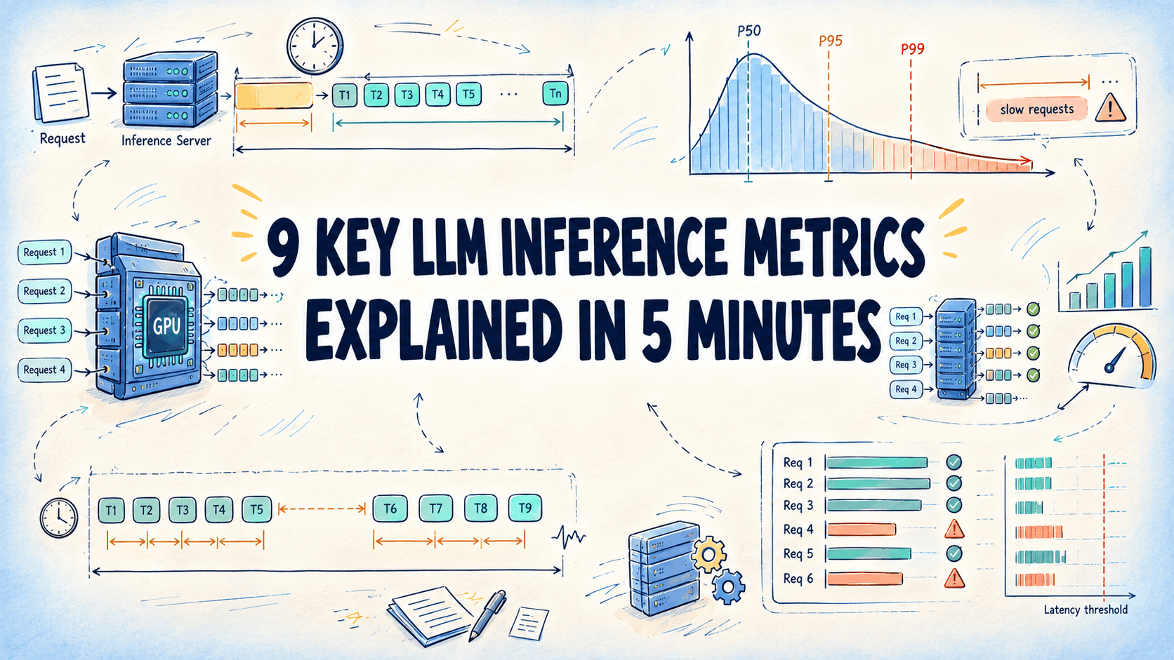
5分钟读懂9个关键LLM推理指标
作者:Bala Priya C,KDnuggets 特约编辑兼技术内容专家,2026 年 11 月 11 日,语言模型栏目
在大语言模型(LLM)应用中,高 Token 吞吐未必能转化为快速的用户体验。首个 Token 可能要等很久才到达,或者后续 Token 流式输出的速度过慢,尤其是在并发负载下。仅凭吞吐量无法反映这些差异。
LLM 推理指标有助于把性能拆解为可度量的组成部分,从最初的响应延迟到 Token 生成速度和整体系统负载。本文介绍九项关键指标、它们的计算公式,以及如何用它们来评估延迟、定位瓶颈并长期跟踪性能:
单请求延迟:首 Token 时间(TTFT)、端到端延迟(E2E)、Token 生成时间、每输出 Token 耗时(TPOT)和 Token 间延迟(ITL)
多请求下的延迟:均值、中位数和尾部百分位数
服务器负载:每秒请求数(RPS)和每秒 Token 数(TPS)
服务质量:有效吞吐(goodput)
我们先从单个请求的时间线开始。
解读请求时间线
下面大多数延迟指标都由四个值定义。值 \( t_{\text{send}} \) 是请求离开客户端的时刻,\( t_{\text{first}} \) 是首个输出 Token 到达的时刻,\( t_{\text{last}} \) 是最后一个输出 Token 到达的时刻,\( N_{\text{out}} \) 是输出 Token 的数量。ITL 还需要每个单独输出 Token 的到达时间 \( t_j \),其中 \( t_1 = t_{\text{first}} \),\( t_{N_{\text{out}}} = t_{\text{last}} \)。
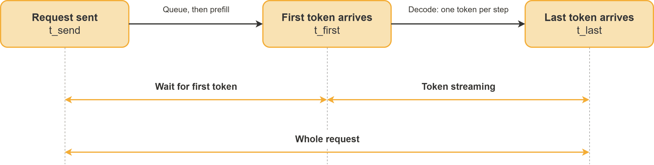
放在时间线上看,这三个时间戳将一次请求切分为两个阶段:
请求时间线:等待首个 Token、Token 流式输出,以及整次请求
在 \( t_{\text{first}} \) 之前,请求可能先在队列中等待,随后服务器执行预填充(prefill),即处理提示词并生成首个 Token。在 \( t_{\text{first}} \) 之后,服务器执行解码(decode),一次一步地输出 Token,通常每步一个 Token。下面的每个延迟指标衡量的都是其中某个阶段,或整个时间跨度。
前六个指标描述的是用户需要等待多久,先看单次请求,再看多次请求。
TTFT 是从发送请求到收到首个输出 Token 之间的延迟。它包含网络传输、在服务器队列中的等待,以及提示词处理步骤,因此会随服务器负载和提示词长度而增加。
\[ \text{TTFT} = t_{\text{first}} - t_{\text{send}} \]
交互式聊天应用最关注这个数字,因为它决定了用户盯着空白屏幕的时长。
端到端(E2E)延迟是总等待时间,从发送请求到收到最后一个 Token。
\[ \text{E2E} = t_{\text{last}} - t_{\text{send}} \]
它是首 Token 等待时间与下一项指标所衡量的流式传输时间之和。
3. Token 生成时间
Token 生成时间是流式输出段的持续时间:即服务器交付首个 Token 之后每一个 Token 所需的时间。
\[ \text{TokenGen} = t_{\text{last}} - t_{\text{first}} = \text{E2E} - \text{TTFT} \]
Token 生成时间随输出 Token 数量增长,因此应使用 TPOT(下文讨论)来评判流的速度,它把这一长度因素分摊掉了。
4. 每个输出 Token 的耗时(Time per Output Token)
TPOT 是首个输出 Token 之后各输出 Token 之间的平均时间。它把 Token 生成时间均匀分摊到首个 Token 之后的各个 Token 上。
\[ \text{TPOT} = \frac{\text{E2E} - \text{TTFT}}{N_{\text{out}} - 1} = \frac{\text{TokenGen}}{N_{\text{out}} - 1} \]
首个 Token 归属于 TTFT,这就是分母为 \( N_{\text{out}} - 1 \) 的原因,也是单 Token 回复的 TPOT 无定义的原因。基准测试工具在细节上并不一致:有些将 TTFT 计入平均值,有些则把 ITL 当作 TPOT 的另一个名称。跨工具比较结果之前,先确认定义。
ITL 是两个连续输出 Token 之间的间隔。一个包含 \( N_{\text{out}} \) 个 Token 的请求有 \( N_{\text{out}} - 1 \) 个间隔,每个间隔各自都是一次独立测量。
\[ \text{ITL}_j = t_{j+1} - t_j, \quad j = 1, \dots, N_{\text{out}} - 1 \]
对于单个请求,其 ITL 值的均值等于其 TPOT。而在 \( R \) 个请求上,这两个平均值对数据的加权方式不同。用 \( N_i \) 表示请求 \( i \) 的输出 Token 数,则平均 ITL 对每个间隔各计一次,平均 TPOT 对每个请求各计一次:
\[ \overline{\text{ITL}} = \frac{\sum_{i=1}^{R} \sum_{j=1}^{N_i - 1} \text{ITL}_{i,j}}{\sum_{i=1}^{R} (N_i - 1)} \qquad \overline{\text{TPOT}} = \frac{1}{R} \sum_{i=1}^{R} \text{TPOT}_i \]
少数长请求会主导第一种平均值,而第二种则让短请求和长请求具有同等权重。ITL 还会保留每一个单独的间隔,流式输出中的卡顿正是在这里显现出来。
6. 均值、中位数与尾部百分位数
延迟因请求而异,因此每个请求的单个数值在大量请求上就构成了一个分布。
均值是所有数值的平均值,会随离群值变动
中位数也称为 P50,是有一半请求小于或等于的数值,反映典型用户的情况
P99 是 99% 的请求小于或等于的数值,体现尾部情况,P90 和 P95 则是较温和的版本
将这三者分别应用于 TTFT、TPOT 和 E2E。
将 \( N \) 个测量值按升序排列为 \( x_{(1)} \le x_{(2)} \le \dots \le x_{(N)} \),最近秩方法给出:
\[ \bar{x} = \frac{1}{N} \sum_{i=1}^{N} x_i \qquad P_k = x_{\left(\left\lceil \frac{k}{100} N \right\rceil\right)} \]
每个百分位数都应基于所有服务器合并后的原始样本计算,因为各服务器 P99 值的平均值并不等于合并流量的 P99。
测量吞吐与有效吞吐
最后三项指标描述的是整个服务器,测量窗口为 \( t_{\text{start}} \) 到 \( t_{\text{end}} \)。
RPS 统计服务器在每秒钟墙上时钟时间内完成的请求数。
\[ \text{RPS} = \frac{N_{\text{completed}}}{t_{\text{end}} - t_{\text{start}}} \]
RPS 忽略了每个请求所承载的工作量,因此只应在提示词与输出长度构成相同的多次运行之间进行比较。
TPS 统计服务器在所有活跃请求上每秒处理的 Token 数。它分为输出形式和输入形式。记 \( N_{\text{prompt},i} \) 为请求 \( i \) 的提示词 Token 数:
\[ \text{TPS}_{\text{out}} = \frac{\sum_{i} N_{\text{out},i}}{t_{\text{end}} - t_{\text{start}}} \qquad \text{TPS}_{\text{in}} = \frac{\sum_{i} N_{\text{prompt},i}}{t_{\text{end}} - t_{\text{start}}} \]
说明所引用的数字采用的是哪种形式,因为长提示、短回复的工作负载可能录得较高的输入 TPS,却只产生少量输出 Token。
有效吞吐(Goodput)是成功完成且满足服务级目标(SLO)的请求速率,vLLM 等服务基准测试就是这样计算的。SLO 是一种延迟限制,例如 TTFT 或 TPOT 的上限,一个请求只有满足每项限制时才计入。DistServe 论文则用该术语表示一种容量:GPU 在其延迟约束内可维持的最大请求速率。将这些限制记为 \( s_{\text{ttft}} \)、\( s_{\text{tpot}} \) 和 \( s_{\text{e2e}} \),请求 \( i \) 为合格的条件是:
\[ \text{TTFT}_i \le s_{\text{ttft}} \;\land\; \text{TPOT}_i \le s_{\text{tpot}} \;\land\; \text{E2E}_i \le s_{\text{e2e}} \]
统计合格请求数并除以时间窗口,即可得到有效吞吐:
\[ \text{Goodput} = \frac{N_{\text{good}}}{t_{\text{end}} - t_{\text{start}}} \]
有效吞吐永远不会超过 RPS,两者之间的差距是至少错过一个目标的请求速率。
推理指标将单个请求拆分为首 Token 等待和流式传输,然后描述服务器在大量请求中的表现,以及其中有多少请求达到你的目标。下表对它们进行了总结:
\( t_{\text{first}} - t_{\text{send}} \)
回复开始所需的时间
\( t_{\text{last}} - t_{\text{send}} \)
整个回复所需的时间
\( t_{\text{last}} - t_{\text{first}} \)
流持续的时间
\( \frac{\text{E2E} - \text{TTFT}}{N_{\text{out}} - 1} \)
Token 平均到达的速度
流式输出是否停滞
P99 对应的 \( x_{(\lceil 0.99 N \rceil)} \)
典型请求与最慢请求的对比
\( \frac{N_{\text{completed}}}{t_{\text{end}} - t_{\text{start}}} \)
每秒完成多少请求
\( \frac{\sum_i N_{\text{out},i}}{t_{\text{end}} - t_{\text{start}}} \)
服务器每秒生成多少 Token
\( \frac{N_{\text{good}}}{t_{\text{end}} - t_{\text{start}}} \)
有多少请求满足所有 SLO
参考资料与延伸学习:
原文较长,译文为节选;译文由英文原文机器翻译,术语按行业惯例统一,可在文末展开原文核对。
查看英文原文(9 Key LLM Inference Metrics Explained in 5 Minutes)
By Bala Priya C, KDnuggets Contributing Editor & Technical Content Specialist on November 11, 2026 in Language Models
A high token throughput doesn't necessarily translate to a fast user experience in a large language model (LLM) application. The first token may take too long to arrive, or subsequent tokens may stream too slowly, especially under concurrent load. Throughput alone doesn't capture these differences.
LLM inference metrics help break performance down into measurable components, from the initial response delay to token generation speed and overall system load. This article covers nine key metrics, their formulas, and how to use them to evaluate latency, identify bottlenecks, and track performance over time:
Per-request latency: time to first token (TTFT), end-to-end latency (E2E), token generation time, time per output token (TPOT), and inter-token latency (ITL)
Latency across many requests: mean, median, and tail percentiles
Server load: requests per second (RPS) and tokens per second (TPS)
Service quality: goodput
We start with the timeline of a single request.
Reading a Request Timeline
Four values define most of the latency metrics below. The value \( t_{\text{send}} \) is the moment the request leaves the client, \( t_{\text{first}} \) is the arrival time of the first output token, \( t_{\text{last}} \) is the arrival time of the last output token, and \( N_{\text{out}} \) is the number of output tokens. ITL also needs the arrival time \( t_j \) of each individual output token, where \( t_1 = t_{\text{first}} \) and \( t_{N_{\text{out}}} = t_{\text{last}} \).
Laid on a timeline, the three timestamps cut a request into two segments:
 Request timeline: wait for first token, token streaming, and whole request
Before \( t_{\text{first}} \), the request may wait in a queue, and then the server runs prefill, which processes the prompt and produces the first token. After \( t_{\text{first}} \), the server runs decode and emits tokens one step at a time, usually one token per step. Each latency metric below measures one of these segments or the whole span.
The first six metrics describe how long a user waits, for one request and then across many.
TTFT is the delay between sending a request and receiving the first output token. It includes network travel, any wait in the server queue, and the prompt-processing step, so it grows with server load and with prompt length.
\[
\text{TTFT} = t_{\text{first}} - t_{\text{send}}
\]
Interactive chat applications watch this number most closely, because it sets how long the user stares at a blank screen.
E2E latency is the total wait, from sending the request to receiving the last token.
\[
\text{E2E} = t_{\text{last}} - t_{\text{send}}
\]
It is the sum of the first-token wait and the streaming time that the next metric measures.
3. Token Generation Time
Token generation time is the duration of the streaming segment: how long the server takes to deliver every token after the first.
\[
\text{TokenGen} = t_{\text{last}} - t_{\text{first}} = \text{E2E} - \text{TTFT}
\]
Token generation time grows with the number of output tokens, so judge the speed of the stream with TPOT (discussed next), which divides that length out.
4. Time per Output Token
TPOT is the average time between output tokens after the first one. It spreads the token generation time evenly over the tokens that follow the first.
\[
\text{TPOT} = \frac{\text{E2E} - \text{TTFT}}{N_{\text{out}} - 1} = \frac{\text{TokenGen}}{N_{\text{out}} - 1}
\]
The first token belongs to TTFT, which is why the denominator is \( N_{\text{out}} - 1 \), and why TPOT is undefined for a reply with a single token. Benchmarking tools disagree on details here: some include TTFT in the average, and some use ITL as another name for TPOT. Confirm the definition before comparing results across tools.
ITL is the gap between two consecutive output tokens. A request with \( N_{\text{out}} \) tokens has \( N_{\text{out}} - 1 \) gaps, and each gap is its own measurement.
\[
\text{ITL}_j = t_{j+1} - t_j, \quad j = 1, \dots, N_{\text{out}} - 1
\]
For one request, the mean of its ITL values equals its TPOT. Across \( R \) requests, the two averages weight the data differently. Writing \( N_i \) for the output tokens of request \( i \), the mean ITL counts every gap once, and the mean TPOT counts every request once:
\[
\overline{\text{ITL}} = \frac{\sum_{i=1}^{R} \sum_{j=1}^{N_i - 1} \text{ITL}_{i,j}}{\sum_{i=1}^{R} (N_i - 1)}
\qquad
\overline{\text{TPOT}} = \frac{1}{R} \sum_{i=1}^{R} \text{TPOT}_i
\]
A few long requests dominate the first average, and the second gives short and long requests equal say. ITL also keeps every individual gap, which is where a stall in the stream shows up.
6. Mean, Median, and Tail Percentiles
Latency varies from request to request, so one number per request becomes a distribution across many requests.
The mean is the average of all values and follows outliers
The median, also called P50, is the value that half of the requests fall at or below and reflects the typical user
P99 is the value that 99% of requests fall at or below and shows the tail, with P90 and P95 as softer versions
Apply all three to TTFT, TPOT, and E2E separately.
With the \( N \) measured values sorted in ascending order as \( x_{(1)} \le x_{(2)} \le \dots \le x_{(N)} \), the nearest-rank method gives:
\[
\bar{x} = \frac{1}{N} \sum_{i=1}^{N} x_i
\qquad
P_k = x_{\left(\left\lceil \frac{k}{100} N \right\rceil\right)}
\]
Compute each percentile from the raw samples of all servers combined, because an average of per-server P99 values is not the P99 of the combined traffic.
Measuring Throughput and Goodput
The last three metrics describe the server as a whole, over a measurement window from \( t_{\text{start}} \) to \( t_{\text{end}} \).
RPS counts the requests the server completes per second of wall-clock time.
\[
\text{RPS} = \frac{N_{\text{completed}}}{t_{\text{end}} - t_{\text{start}}}
\]
RPS ignores how much work each request carries, so compare it only across runs with the same mix of prompt and output lengths.
TPS counts the tokens the server processes per second across all active requests. It has an output form and an input form. Writing \( N_{\text{prompt},i} \) for the prompt tokens of request \( i \):
\[
\text{TPS}_{\text{out}} = \frac{\sum_{i} N_{\text{out},i}}{t_{\text{end}} - t_{\text{start}}}
\qquad
\text{TPS}_{\text{in}} = \frac{\sum_{i} N_{\text{prompt},i}}{t_{\text{end}} - t_{\text{start}}}
\]
State which form a quoted number uses, since a workload with long prompts and short replies can post a high input TPS while producing few output tokens.
Goodput is the rate of successfully completed requests that meet your service-level objectives (SLOs), which is how serving benchmarks such as vLLM compute it. An SLO is a latency limit, such as a ceiling on TTFT or TPOT, and a request counts only when it satisfies every limit. The DistServe paper uses the term for a capacity instead: the maximum request rate a GPU sustains within its latency constraints. Writing \( s_{\text{ttft}} \), \( s_{\text{tpot}} \), and \( s_{\text{e2e}} \) for those limits, request \( i \) is good when:
\[
\text{TTFT}_i \le s_{\text{ttft}} \;\land\; \text{TPOT}_i \le s_{\text{tpot}} \;\land\; \text{E2E}_i \le s_{\text{e2e}}
\]
Counting the good requests and dividing by the window gives goodput:
\[
\text{Goodput} = \frac{N_{\text{good}}}{t_{\text{end}} - t_{\text{start}}}
\]
Goodput never exceeds RPS, and the gap between them is the rate of requests that missed at least one target.
Inference metrics split one request into a first-token wait and a stream, then describe how a server performs across many requests and how many of them meet your targets. The table below summarizes them:
\( t_{\text{first}} - t_{\text{send}} \)
How long the reply takes to start
\( t_{\text{last}} - t_{\text{send}} \)
How long the whole reply takes
\( t_{\text{last}} - t_{\text{first}} \)
How long the stream lasts
\( \frac{\text{E2E} - \text{TTFT}}{N_{\text{out}} - 1} \)
How fast tokens arrive on average
Whether the stream stalls
\( x_{(\lceil 0.99 N \rceil)} \) for P99
How typical and slowest requests compare
\( \frac{N_{\text{completed}}}{t_{\text{end}} - t_{\text{start}}} \)
How many requests complete per second
\( \frac{\sum_i N_{\text{out},i}}{t_{\text{end}} - t_{\text{start}}} \)
How many tokens the server produces per second
\( \frac{N_{\text{good}}}{t_{\text{end}} - t_{\text{start}}} \)
How many requests meet every SLO
References and Further Learning:
Bala Priya is a developer, educator, and technical writer based in India. She writes about programming, data science, machine learning, and AI, with a focus on making complex technical ideas practical and approachable. She creates tutorials, how-to guides, and deep dives that help developers build, solve problems, and understand complex technical concepts. Her technical interests include LLM applications, agentic AI, graph algorithms, computer vision, explainable AI, and ML systems. When she’s not writing or coding, Bala is usually reading classic literature, epic fantasy, or speculative fiction. She also enjoys talking about books, learning new things, and sharing what she learns with the developer community.
原文为英文,正文由自动抓取并保留原文。
原文发布于 KDnuggets(9 Key LLM Inference Metrics Explained in 5 Minutes),标题、摘要与正文由机器翻译,术语按行业惯例统一,未经人工逐句校订。