连续批处理在 vLLM 中比静态与动态最高快 2.91 倍

我发现的核心问题是:输出长度的差异很关键。当各个请求在不同时间结束时,连续批处理(continuous batching)可以填补空出来的位置;当它们同时结束时,就没有什么可以回收的。可以把一个批次想象成一间会议室。如果人们在不同时间离开,连续批处理就能在座位空出时逐一填上。如果所有人同时离开,那就没什么可填的了。
本文面向谁,以及你能获得什么
任何正在运行推理服务器、或正在选型推理服务器的人,以及看到过连续批处理(continuous batching)带来 10 倍或 20 倍收益说法的人,都能从本文中获益。
为什么一个 decode 步骤服务 1 个还是 32 个序列,成本都一样
在理解各种批处理策略之前,我发现把 transformer 的生成过程拆分为 prefill 和 decode 很有帮助。Prefill 在一次前向传播中读取提示词,因此其成本随提示词长度增长,并让 GPU 有大量算术工作可做。Decode 则不同:每一步每个序列只产生一个 Token,而每一步都必须重新读取模型权重。这一区别很重要,因为我原本以为更大的 decode 批次会让每一步明显变慢。然而,我的测量结果并没有显示出这一点。
bfloat16 格式的 Qwen2.5-7B-Instruct 权重约为 15.2 GB。DGX Spark 中的 GB10 提供 273 GB/s 的标称内存带宽,因此读取一遍这些权重的理论下限约为 55.7 ms。我实测 batch 1 时每步为 78.05 ms,约为该下限的 1.4 倍。换算下来是 194.7 GB/s,即标称带宽的 71%,但我不会把它当作 DRAM 效率的测量结果。解码要做的事不只是读取权重,所以我只把它用作一致性检查。对我来说有用的类比是一辆开往仓库的卡车。无论我是取回一个订单,还是把好几个订单装到同一辆卡车上,这一趟的时间都大致相同。批处理让更多序列能够使用我已经不得不取回的权重。
我们来看看当我增大 batch 后发生了什么。
从 batch 1 提升到 batch 32 使总吞吐提升了 26.7 倍,而实测的流式 Token 间隔基本持平。batch 1 时我看到 78.05 ms,batch 32 各次运行平均为 74.77 ms。这个结果令人意外,因为更大的 batch 在 Token 之间并没有变慢。
然而,这些是客户端侧的 Token 间隔,而非 GPU 迭代计时。batch 32 的数字还基于 3 次运行、每次 512 个请求,而 batch 1 只用了 1 次 16 个请求的运行,所以我不会对这约 4% 的差异做任何解读。在一个解码步骤中服务 32 个序列,并没有让该步骤比服务 1 个序列明显更慢。两种情况仍然都要读取同样的 15.2 GB 权重。
就单请求成本而言,在 batch 为 32 的情况下,一个请求从准入到生成首个 Token 等待了约 2.8 秒,而单独一个请求只需 121 ms。这一延迟来自批处理和预填充,而非 Token 之间的解码变慢。在 128 个输出 Token 上,这段额外等待使每条序列的有效吞吐从 12.76 tokens/s 降至 10.66 tokens/s,下降了 16%。换言之,代价出现在流式输出开始之前,而不是后续 Token 之间。
一旦请求进入流式输出,我在 batch 为 32 时并未观察到 Token 输出变慢。
图 1。预填充受算力约束,并随提示长度增长;解码则每一步都要重新读取全部 15.2 GB 权重,与批大小无关。图片由作者提供。
这就是我会带入后续批处理策略中的取舍。就解码而言,让某个批处理槽位空着并不能省下读取权重的开销。因此,我接下来关注的是让这些槽位保持占用,同时不让预填充和排队延迟增长到用户无法忍受的程度。
我保持工作负载固定不变:八个请求、四个槽位,输出长度也相同。我只改了一件事:允许等待中的请求何时开始。正是这个小小的改动带来了大部分差异。
图 2。八个请求,输出长度分别为 3、9、2、7、5、12、4 和 6 步,四个槽位,三种准入规则。静态(static)方式在 32 步内完成,其占用的槽位时间中有 42.9% 处于空闲;连续(continuous)方式在 26 步内完成,且没有空闲。动画中的每个计数器都由模拟计算得出,而非手工输入。图片由作者提供。
静态批处理会凑齐恰好 B 个请求,将它们放在一起运行,并等待每个请求都结束后才启动下一批。如果 32 个请求同时开始,其中 31 个在 40 个 Token 后完成,而有一个要跑到 700,那么这 31 个槽位会在 660 个解码步骤中一直闲置。这大致就是 model.generate() 在填充批次(padded batch)上的情况,在简单的服务系统中也会出现。
图 3。31 个请求在第 40 步完成,它们的槽位一直被占用(斜线阴影),直到最慢的那个成员在第 700 步完成:20,460 个闲置槽位-步,占该批次槽位时间的 91%。直到这时才会收集下一批 32 个请求。这是对所举示例的示意,并非实测结果。图片由作者提供。
动态批处理增加了一个计时器。如果队列没有填满,批次仍可在超时后出发。我原本以为这能比实际效果更多地解决利用率问题。它有助于改善排队延迟,这很有用,但并不会改变批次开始之后的情况。换句话说,那个长请求仍然会让已完成的槽位闲置。
图 4。动态批处理器按大小触发(左)或按超时触发(右)。图片由作者提供。
连续批处理改变了调度的单位。每个解码步骤之后,调度器都会检查是否有序列完成,并立即把该槽位交给等待中的请求。我把它类比成理发店。静态批处理会让每把椅子都保留到最后一个顾客离开;连续批处理则是一旦有椅子空出来就马上安排新顾客坐下。
沿用同一个例子,这 31 个被释放的槽位可以在下一个解码步骤就承接新工作,而不是继续闲置 660 步。GPU 本身并没有变快。只是已完成的序列不再占用容量。
图 5。与图 3 相同的 32 个请求、同样那个慢请求,在连续规则下。每个席位在释放后经过一个解码迭代就被重新填满,因此原本静态空置、什么都没做的 20,460 个槽位步,转而用于服务新请求。新占用者是无限抽取进来的,因为它们被接纳时输出长度尚不可知,而这正是下一节要讨论的问题。此为示意,不是实测。图片由作者提供。
这正是 Orca 的迭代级调度(Yu 等,OSDI 2022)的核心思想:活跃批次变成一组不断滚动的序列,而不是一个固定的分组。
为什么内存管理很重要
我最初把这主要当作一个调度问题,但结果它比这更大。每个活跃序列还拥有一个 KV 缓存,而它的最终长度事先未知。如果这块内存按一整块连续区域预留,已完成的请求就会留下难以复用的空洞。
图 6。在连续 KV 预留下,一个被释放的槽位留下一个空洞,下一个请求未必放得进去。图片由作者提供。
PagedAttention(Kwon 等,SOSP 2023)通过以更小的块来管理 KV 缓存内存,解决了这个问题。它是一项内存管理技术,不是调度策略,但两者协同工作。在解读吞吐量说法时,这一区分很重要。例如,Anyscale 报告的 23× 结果既包含 PagedAttention 的效果,也包含连续批处理的效果。
市场上在提供的是什么
许多厂商对不同的类型使用相同的命名。Triton 的“dynamic batching”是请求级批处理,而 NVIDIA 的“in-flight batching”就是大多数人所说的连续批处理。
--max-num-batched-tokens
在 V1 中默认开启;使用 --no-enable-chunked-prefill 可禁用
--max-concurrent-requests(默认 128)
--max-batch-total-tokens、--max-batch-prefill-tokens
--waiting-served-ratio(默认 0.3)控制暂停运行中的请求
max_batch_size(引擎构建时,默认 2048)
max_num_tokens(引擎构建时,默认 8192)
capacity_scheduler_policy:GUARANTEED_NO_EVICT(默认)、MAX_UTILIZATION、STATIC_BATCH
连续批处理 + RadixAttention
--chunked-prefill-size(-1 表示禁用)
preferred_batch_size、max_batch_size
我最初以为 Triton 的动态批处理器会更接近连续批处理。事实上并非如此。它通过 max_queue_delay_microseconds 来决定一个批次何时开始,该参数默认值为 0,然后从头到尾运行该批次。实践中,把它放在 LLM 前面得到的是这里描述的中间策略,而非连续批处理。
TensorRT-LLM 在一个配置中暴露了全部三种策略,从而让这一区分更加清晰。STATIC_BATCH 是静态批处理,为兼容旧用法而保留,而 GUARANTEED_NO_EVICT 和 MAX_UTILIZATION 则体现了准入控制的权衡。在比较这些系统时,我会记住这套术语。
我在一台配备 GB10 和 128 GB 统一 LPDDR5X 内存的 DGX Spark 上运行了测试。模型是 bfloat16 精度的 Qwen2.5-7B-Instruct,由一个固定版本的 vLLM 镜像提供服务,且前缀缓存已禁用。我还停掉了另外 2 个 vLLM 租户,这样就没有其他东西会占用 GPU。
原文较长,译文为节选;译文由英文原文机器翻译,术语按行业惯例统一,可在文末展开原文核对。
查看英文原文(Continuous Batching Beats Static and Dynamic by Up to 2.91× in vLLM)
The main thing I found is that output-length variation matters: when requests finish at different times, continuous batching can refill the gaps; when they finish together, there is little to recover. Think of a batch like a meeting room. If people leave at different times, continuous batching fills each empty seat as it opens. If everyone leaves together, there is nothing to refill.
Who this is for, and what you'll take away
Anyone who is running an inference server, or choosing one, and who has seen claims of 10× or 20× gains from continuous batching can find this article beneficial.
Why a decode step costs the same whether it serves 1 or 32
Before the batching policies make sense, I found it useful to separate transformer generation into prefill and decode. Prefill reads the prompt in one forward pass, so its cost grows with prompt length and gives the GPU plenty of arithmetic work. Decode is different: it produces one token per sequence per step, and each step has to read the model weights again. That distinction is important because I initially expected a larger decode batch to make each step noticeably slower. However, it does not show this in my measurements.
Qwen2.5-7B-Instruct in bfloat16 has about 15.2 GB of weights. The GB10 in the DGX Spark provides 273 GB/s of rated memory bandwidth, so reading those weights once gives a theoretical floor of about 55.7 ms.: I measured 78.05 ms per step at batch 1, about 1.4× that floor. That works out to 194.7 GB/s, or 71% of rated bandwidth, but I would not treat that as a DRAM-efficiency measurement. Decode does more than read weights, so I use it only as a consistency check. The useful comparison for me is a truck going to a warehouse. The trip takes roughly the same time whether I bring back one order or load several orders onto the same truck. Batching lets more sequences use the weights I already had to fetch.
Let's look at what happened when I increased the batch.
Moving from batch 1 to batch 32 increased total throughput by 26.7×, while the measured gap between streamed tokens stayed roughly flat. I saw 78.05 ms at batch 1 and 74.77 ms averaged across the batch-32 runs. This result is a surprise as the larger batch was not slower between tokens.
However, these are client-side inter-token gaps, not GPU iteration timings. The batch-32 number is also based on 3 runs of 512 requests, while batch 1 used 1 run of 16 requests, so I would not make anything of the roughly 4% difference. Serving 32 sequences in a decode step did not make that step materially slower than serving 1. Both cases still had to read the same 15.2 GB of weights.
Regarding per-request cost, a request in the batch-32 case waited about 2.8 seconds from admission to first token, compared with 121 ms for a lone request. That delay comes from batching and prefill rather than from slower token-to-token decoding. Across 128 output tokens, that extra wait reduced effective per-sequence throughput from 12.76 tokens/s to 10.66 tokens/s, a 16% drop. In other words, the penalty appeared before streaming began, not between later tokens.
Once a request was streaming, I did not observe slower token delivery at batch 32.
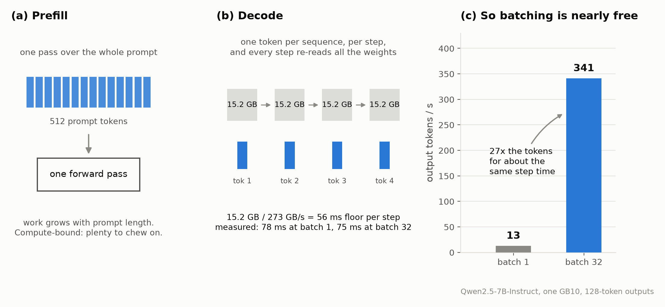
Figure 1 . Prefill is compute-bound and scales with prompt length; decode re-reads all 15.2 GB of weights every step regardless of batch size. Image by author.
That is the trade I would carry into the batching policies that follow. For decode, leaving a batch slot unused does not save the weight-read cost. I would therefore focus next on keeping those slots occupied without letting prefill and queueing delay grow beyond what users can tolerate.
I kept the workload fixed: eight requests, four slots, and the same output lengths. I changed only one thing: when a waiting request was allowed to start. That small change produced most of the difference.
Figure 2 . Eight requests with output lengths 3, 9, 2, 7, 5, 12, 4, and 6 steps, four slots, three admission rules. Static finishes in 32 steps with 42.9% of its held slot-time idle; continuous finishes in 26 with none. Every counter in the animation is computed from the simulation, not typed in. Image by author.
Static batching collects exactly B requests, runs them together, and waits for every request to finish before starting another batch. If 32 requests start together, 31 finish after 40 tokens, and one runs to 700, those 31 slots sit unused for 660 decode steps. That is roughly what happens with model.generate() on a padded batch, and it also appears in simple serving systems.
Figure 3 . Thirty-one requests finish at step 40 and their slots stay held (hatched) until the slowest member finishes at step 700: 20,460 idle slot-steps, 91% of the batch's slot-time. Only then is the next batch of 32 collected. An illustration of the stated example, not a measurement. Image by author.
Dynamic batching adds a timer. If the queue does not fill, the batch can still leave after a timeout. I expected this to solve more of the utilization problem than it did. It helps queueing latency, which is useful, but it does not change what happens after the batch starts. In other words, the long request can still keep finished slots idle.
Figure 4 . A dynamic batcher fires on size (left) or on timeout (right). Image by author.
Continuous batching changes the unit of scheduling. After every decode step, the scheduler checks whether a sequence finished and immediately gives that slot to a waiting request. I think of it like a barbershop. Static batching keeps every chair reserved until the last customer leaves; continuous batching seats someone new as soon as one chair opens.
Using the same example, the 31 freed slots can accept new work on the next decode step instead of remaining idle for 660 steps. The GPU is not faster. Finished sequences simply stop occupying capacity.
Figure 5 . The same 32 requests and the same slow one as Figure 3, under the continuous rule. Every seat is refilled one decode iteration after it frees, so the 20,460 slot-steps static spent holding nothing are serving new requests instead. The new occupants are drawn without an end because their output lengths are not known when they are admitted, which is the problem the next section is about. An illustration, not a measurement. Image by author.
This is the main idea behind Orca's iteration-level scheduling (Yu et al., OSDI 2022): the active batch becomes a rolling set of sequences rather than a fixed group.
Why memory management matters
I initially treated this as mostly a scheduling problem but it turned out to be something bigger than that. Each active sequence also owns a KV cache, and its final length is unknown in advance. If that memory is reserved as one contiguous block, finished requests can leave gaps that are awkward to reuse.
Figure 6 . With contiguous KV reservations, a freed slot leaves a hole the next request may not fit into. Image by author.
PagedAttention (Kwon et al., SOSP 2023) addresses that problem by managing KV-cache memory in smaller blocks. It is a memory-management technique, not a scheduling policy, but the two work together. That distinction matters when interpreting throughput claims. For example, Anyscale's reported 23× result includes the effects of PagedAttention as well as continuous batching.
What is being offered on the market
Many entities are using the same naming for different types. Triton’s “dynamic batching” is request-level batching, while NVIDIA’s “in-flight batching” is what most people call continuous batching.
--max-num-batched-tokens
on by default in V1; --no-enable-chunked-prefill to disable
--max-concurrent-requests (default 128)
--max-batch-total-tokens, --max-batch-prefill-tokens
--waiting-served-ratio (default 0.3) governs pausing running requests
max_batch_size (engine build, default 2048)
max_num_tokens (engine build, default 8192)
capacity_scheduler_policy: GUARANTEED_NO_EVICT (default), MAX_UTILIZATION, STATIC_BATCH
continuous batching + RadixAttention
--chunked-prefill-size (-1 disables)
preferred_batch_size, max_batch_size
I initially expected Triton’s dynamic batcher to behave more like continuous batching. Indeed, it does not. It decides when a batch starts using max_queue_delay_microseconds, which defaults to 0, and then runs that batch from end to end. In practice, putting it in front of an LLM gives you the middle policy described here, not continuous batching.
TensorRT-LLM makes the distinction clearer by exposing all three policies in one configuration. STATIC_BATCH is static batching, retained for legacy use, while GUARANTEED_NO_EVICT and MAX_UTILIZATION represent the admission-control trade-off. That is the terminology I would keep in mind when comparing these systems.
I ran the test on one DGX Spark with a GB10 and 128 GB of unified LPDDR5X. The model was Qwen2.5-7B-Instruct in bfloat16, served by one pinned vLLM image with prefix caching disabled. I also stopped the other 2 vLLM tenants so nothing else could use the GPU.
All 3 policies hit the same running server through one asyncio client. That mattered to me because I wanted the admission logic to be the only thing changing; the engine, kernels, memory manager, and hardware stayed fixed. I used 4 checks to keep the comparison honest.
In-flight parity. Continuous batching was capped at 32 requests in flight, matching static batching at B=32. Peak concurrency reached exactly 32 for both through the burst ladder, except where offered load was too low to fill every slot. This means I was comparing scheduling, not different concurrency limits.
Identical work. Every policy replayed the same seeded workload. Each trace contained 512 requests with 512-token prompts and prescribed output lengths, using ignore_eos so every request had to emit its assigned count. If even 1 completion came back short, the run failed instead of quietly making throughput look better. That check caught 1 dropped 512-token request, so I discarded that run and repeated it.
A zero-variance control. I included a zero-variance control called const128. Every request there produces exactly 128 tokens. I expected all 3 policies to agree because nothing finishes early enough for continuous batching to reclaim a slot. That control became the simplest way to tell whether the rig itself was lying.
I ran 3 repeats for every static and continuous cell and report the spread. The dynamic arm gets 1 confirmation run per burst trace because I use it only to check whether it lands on static.
The dataset consists of five traces, each containing 512 requests with 512-token prompts. The traces differ only in reply length. For variable-length traces, reply lengths are sampled from an exponential distribution with a mean of 128 tokens and capped at the maximum specified by each trace. The exception is const128, where every reply is fixed at 128 tokens.
Traffic it stands in for
every reply exactly 128 tokens
nothing real; this is the control
exponential, clipped at 32
short replies under a tight token limit
exponential, clipped at 128
mixed lengths, moderately ragged
exponential, clipped at 512
exponential, clipped at 1536
chat traffic with the cap barely binding
I quantify the variation in reply lengths using the coefficient of variation (CV), defined as the standard deviation divided by the mean. A CV of 0 indicates that all replies have the same length, while a CV near 1 indicates substantial variation. This matters for continuous batching because its benefits depend on requests finishing at different times.
Two caveats are worth noting. First, the cap1536 limit has little effect because the longest sampled reply is only 790 tokens. As a result, the two highest-cap traces have similar distributions. Second, reducing the cap affects both the variance and the mean reply length, so this experiment does not isolate variance alone. To ensure fair comparisons, I compare batching policies only within the same trace, rather than across traces.
I started with const128 because I wanted to see whether the setup could falsify itself. With all 512 requests producing exactly 128 tokens, every sequence finishes on the same decoding step. There is no ragged tail and therefore no idle slot for continuous batching to reclaim.
Output tokens/s (mean of 3)
Continuous, capped at 32
I expected the 3 policies to converge, and they did. The static repeats varied by 0.30%, and continuous by 0.42%; both are inside the 5% tolerance I set beforehand. What caught my attention was not that continuous batching won nothing here, but that it won nothing for the right reason. The scheduler is useful when completion times diverge. On this trace, they do not.
Experiment A: How output-length variability affects continuous batching throughput
Within each rung, all three batching policies processed the same trace with a 32-request in-flight limit. Across rungs, both the mean output length and its variability changed, so the most meaningful comparison is the continuous-to-static throughput ratio within each rung: 1.00×, 1.15×, 1.40×, 2.60×, and 2.91×.
What surprised me was how sharply the benefit increased as output lengths became more variable. When every request generated the same number of tokens, continuous batching provided no measurable improvement. At the highest-variability rung, however, it delivered 2.91× the throughput of static batching.
I expected the improvement to increase gradually. Instead, the largest jump occurred between CV 0.58 and 0.94, where the speedup rose from 1.40× to 2.60×. With only five workloads, I cannot determine exactly how the gain changes within that interval, but the results suggest that continuous batching becomes particularly valuable when request completion times differ substantially.
Figure 7. Panel (a): throughput per policy at each rung, dynamic drawn dashed on static because the two coincide everywhere; dynamic is one run per rung, static and continuous means of three. Panel (b): the ratio, which is what compares across rungs, rising 1.00 to 2.91. Heights in (a) do not compare between rungs, because a tighter cap lowers mean and spread together, so each x label carries both. Image by author.
Absolute throughput should only be compared within each trace, since workloads differ in output length and total work.
Dynamic batching performed almost identically to static batching under burst arrivals, with a maximum difference of just 0.26%. All 512 requests arrived at once, so batches filled before the timeout mattered. This shows that timeout tuning has little effect when the queue is consistently full.
Figure 8. End-to-end latency, p50 with a whisker to p99. Under a burst this largely restates throughput in seconds, since latency is dominated by queue position. Read it for the p50-to-p99 spread, which says how evenly the wait is shared. Image by author.
I also checked the mechanism directly. For static batches of 32, I calculated the decode slots left idle while shorter sequences waited for the longest sequence to finish.
Figure 9. Counting the slots static wastes, using only the trace and no GPU, predicts what static actually gave up. Both are zero at zero variance and both grow with the tail. They are different quantities and are not required to match. Image by author.
Predicted idle-slot waste increased alongside measured throughput loss: 11.5% vs. 13.0%, 37.1% vs. 28.5%, 72.4% vs. 61.5%, and 75.1% vs. 65.6%. Although these values differ because they measure decode-slot waste and end-to-end throughput, their similar trends suggest that idle slots are the main cause of the performance loss.
I initially expected timeout tuning to matter more. On the most ragged trace, I changed the dynamic-batching timeout from 50 ms to 500 ms under Poisson arrivals of 2.0 requests per second.
Figure 10. Poisson arrivals at 2.0 requests per second. A tenfold change in the dynamic timeout, 50 ms against 500 ms, changes nothing, because arrivals outrun service by about 2.4 times and the backlog never clears. Continuous, admitting on arrival, reaches first token in 0.26 s against 155.83 s. Image by author.
Increasing the timeout from 50 ms to 500 ms barely affected performance. Throughput remained around 104 tokens/s (0.04% change), while median time-to-first-token increased slightly from 155.83 to 156.10 seconds (0.17%). This happened because requests arrived at 2.0 requests/s, roughly 2.4× the server's capacity of 0.85 requests/s. The resulting backlog kept batches nearly full, making timeout tuning ineffective. Although all six runs formed 17 batches instead of 16 perfectly full ones, dynamic batching still behaved much like static batching.
Continuous batching made a much larger difference, reaching 220.0 tokens/s and reducing median time-to-first-token to 0.26 seconds, approximately 600× lower than dynamic batching.
To see whether timeout tuning mattered under lighter traffic, I repeated the experiment at 0.25 requests/s, using 128 requests and one run per setting. I treat this as a preliminary check rather than a reliable tail-latency measurement.
Here, the timeout behaved as expected. Increasing it from 50 ms to 500 ms reduced the batch count from 33 to 32, but increased median time-to-first-token by 0.276 seconds, with almost no throughput improvement (0.01 tokens/s). This makes sense because arrivals, not server capacity, limited throughput. However, the 5.2-second p99 difference is too large to attribute confidently to the timeout change based on a single 128-request run.
The takeaway is that timeout tuning matters mainly when the queue occasionally runs dry, and even then, it may increase latency without meaningful throughput gains. Continuous batching had a much larger impact on uneven workloads, reaching 2.91× static throughput.
For future experiments, I would focus on the sharp increase in speedup between CV 0.58 and 0.94, rather than further timeout tuning.
Experiment B: Decomposing LLM serving speedups: engine vs. scheduler
Anyscale's reported 23× speedup combines improvements from the inference engine, memory management, and scheduling. I wanted to isolate their contributions using the same workload.
I ran the cap1536 trace through three configurations, changing one component at a time. The HuggingFace baseline used generate at B=32, matching vLLM's static batching limit and admission rule. The baseline was averaged over three runs (within 0.02% variation), while the other results came from Experiment A.
The total improvement was 3.86×: switching from HuggingFace to vLLM with static batching gave 1.33×, while enabling continuous batching on the same engine added another 2.91×. Surprisingly, scheduling contributed more than the engine change.
This does not contradict Anyscale's 23× result, which used OPT-13B on an A100 rather than Qwen2.5-7B on a GB10. Configuration also matters: increasing continuous batching's in-flight limit from 32 to 64 raised throughput to 415.0 tokens/s, or 5.10× over the baseline. I therefore kept both policies capped at 32 for a fair comparison.
The HuggingFace baseline also revealed substantial wasted computation. It generated 260,864 token positions to produce just 64,908 useful tokens, leaving 75.1% as surplus padding. vLLM static batching eliminated this padding by stopping each sequence at its token limit, but finished requests still held their batch slots. Continuous batching removed that remaining inefficiency by immediately admitting new requests into freed slots. The padding fraction also matched the trace-derived idle-slot fraction (0.75118), confirming consistency between the workload and execution.
I also attempted a fourth configuration using HuggingFace's native continuous batching in transformers 5.6.0. Although it initialized and accepted requests, it produced no completions within 900 seconds and hung during shutdown. I stopped the attempt, so I could not measure scheduling gains independently of vLLM's kernels.
Figure 11. The same trace through three stacks, changing one thing at a time. The engine is worth 1.33×; the admission rule on that same engine is worth 2.91×. Rung 4, HuggingFace-native continuous batching, produced no number and is reported as a failed attempt. Image by author.
So my result is fairly simple: the engine helped, but the admission rule helped more on this trace. Next, I would measure the same decomposition on several traffic shapes to see when that ordering changes.
What caught my attention was how much the result depended on the traffic, not the scheduler itself. I expected continuous batching to help broadly. Instead, its value tracked 2 things I can measure from production logs: output-length variance and whether the queue empties.
Figure 12. First, I would measure the coefficient of variation of completion tokens. At 0, continuous batching gave me 1.00× because every sequence finished together. Around 0.6, the gain was about 1.4×. Near 1.0, which resembles an unbounded exponential and is closer to chat traffic, it approached 3×.
Continuous batching does not make the GPU faster; it improves utilization by admitting new requests as soon as others finish. When all requests finish together, there are no idle slots to reclaim.
Queue behavior also matters. When the queue remained full, dynamic batching behaved like static batching because the timeout had little effect. Even under lighter traffic, continuous batching reduced median first-token latency from roughly 10 seconds to under a second.
This also puts Anyscale's 23× claim into perspective. On my setup, the scheduler contributed 2.91×, the engine 1.33×, and the combined naive-to-vLLM improvement reached 3.86×. With uniform output lengths, the scheduler provided no gain.
These results are limited to one model on a single GB10 GPU, using synthetic output lengths and fixed 512-token prompts. Since changing the output cap affected both mean length and variance, comparisons were made only within the same trace. Whether the same gains hold across other hardware remains untested.
For anyone evaluating an inference stack, I would start with two metrics from production logs: output-length variability and how often the request queue empties. Together, they provide a practical starting point for estimating the value of continuous batching.
There are five especially important points to highlight:
1. Continuous batching improves utilization, not raw GPU compute speed. It allows new sequences to occupy slots released by completed requests.
2. Output-length variability is a major determinant of benefit. The measured improvement ranged from 1.00× with uniform lengths to 2.91× with highly variable lengths.
3. Dynamic batching and continuous batching are different. Dynamic batching improves when a batch begins; continuous batching changes the active batch while generation is underway.
4. Schedulers and memory managers solve complementary problems. Continuous batching controls request admission; PagedAttention helps make efficient KV-cache allocation possible.
5. Headline benchmarks must be decomposed carefully. The author's observed 3.86× improvement included a 1.33× engine improvement followed by a 2.91× scheduling improvement, on one fixed workload and hardware setup.
References and resources
Qwen2.5-7B-Instruct (the served model in every run). Qwen team · HF · License apache-2.0.
No dataset is load-bearing here. All output lengths are synthetic, drawn from a seeded exponential; the generator is in the repo. For reference, vLLM's own throughput benchmark uses ShareGPT_Vicuna_unfiltered, whose card declares apache-2.0, though the underlying text is scraped conversation and that declaration is the uploader's rather than the original speakers'.
Orca: A Distributed Serving System for Transformer-Based Generative Models (iteration-level scheduling, the origin of continuous batching). Yu, Jeong, Kim, Kim, Chun · USENIX OSDI 2022, pp. 521-538 · paper.
Efficient Memory Management for Large Language Model Serving with PagedAttention. Kwon, Li, Zhuang, et al. · SOSP 2023 · arXiv:2309.06180 · License CC BY 4.0.
Taming Throughput-Latency Tradeoff in LLM Inference with Sarathi-Serve (chunked prefill). Agrawal, Kedia, Panwar, et al. · OSDI 2024 · arXiv:2403.02310 · License: arXiv perpetual non-exclusive.
vLLM engine arguments and optimization guide · engine args · optimization.
Text Generation Inference launcher reference · docs.
TensorRT-LLM performance tuning guide · max_batch_size and max_num_tokens · runtime flags.
SGLang server arguments · server_args.py.
Triton Inference Server batchers · docs.
How machines make sense of sentence structure: Combinatory Categorial Grammar
June 2, 202511 min read
Enterprise Document Intelligence [Vol.1 #5ter] - Table cells, OCR, captions, headings: cloud-grade structure, running on your own machine. No key, no per-page bill, nothing leaves the building
June 13, 202616 min read
Locate the reasoning by detecting the conclusions
October 28, 20219 min read
A reproducible 100-step LoRA fine-tuning run for OpenVLA, with dataset checks, Colab setup, training metrics, and W&B evidence.
July 21, 202612 min read
October 11, 202611 min read
April 22, 202410 min read
An example of using both popular machine learning packages in R to predict bike sharing demand
January 8, 202110 min read
In this article, we explore how we can, and do, regularize and control the complexity of the models we learn through Bayesian prior...
February 1, 20219 min read
So, you are a data scientist? But I thought you worked in marketing!
August 21, 20206 min read
原文为英文,正文由自动抓取并保留原文。
原文发布于 Towards Data Science(Continuous Batching Beats Static and Dynamic by Up to 2.91× in vLLM),标题、摘要与正文由机器翻译,术语按行业惯例统一,未经人工逐句校订。