Qini 奖励错误增益模型时,应改用双重稳健评分
如果你的增益指标将一个不完美的模型排在真实处理效应排名之上,会怎样?在一个我们知道答案的模拟中,Qini 恰恰会这样做,而遵循它的推荐意味着选择一个真实因果增益更低的排名。
让我们从经典的增益问题开始。假设一家公司需要决定向哪些客户发送营销信息。客户的最佳排名将基于向他们发送营销信息所带来的预期收益,这取决于我们试图推动他们采取的行动的价值,以及由于收到该信息而导致采取这一行动的概率变化。当然,公司并不知道这些概率,因此它使用基于其估计值的不完美排名。
让我们设想一种假设情况:我们知道真实概率,这意味着我们知道就沟通效率而言客户的真正完美排名。假设我们决定将其与基于对这些概率的估计值的不完美排名进行比较。有趣的是——事实证明,Qini 指标(常用于增益测量,后文将进一步描述)会给不完美排名打出更好的分数。这怎么可能呢?
在本文中,Qini 和 IPW 被校准为在一个参考点上与 DR 匹配:即更高选择性、seed-42 留出集中的真实 CATE 排名。这些常数对所有学习器、bootstrap 重采样、分配策略和调参结果保持不变。这会使参考分数对齐,但不会调整混杂因素,也不会改变某个指标内模型的排序。在此示例中,校准后的 Qini 仍偏好 Linear DR 而非真实 CATE 排名,而已知因果增益则偏好真实 CATE。校准公式见下文。
原因在于,仅使用一个能够解释混杂因素的因果模型往往是不够的。如果处理分配依赖于客户特征,我们还需要调整用于评估该因果模型的指标,因为 Qini 指标仍可能包含选择偏差。
在本文中,我们将完整梳理我们尝试度量因果效应的整个演进过程——从提升柱状图(uplift bars),到 Qini 指标,再到用 IPW 和双重稳健得分(doubly robust scores)来评估模型。我们将使用从 S learner 到 DML learner 的六种常见学习器,并考察在不同混杂程度下我们如何评估它们的估计结果。
对于给定的处理 T(一条营销信息)和结果 Y(客户的实际购买),客户的条件平均处理效应(CATE)由下式给出:
τ(x)=E[Y(1)−Y(0)∣X=x]。
CATE 可以理解为具有特征画像 x 的某位客户的平均处理效应(ATE)。它可用于客户定向,因为高 CATE 表明该处理对这位客户的效果更强。需要特别说明的是——这并不意味着高 CATE 的客户具有最高的结果值或采取某种行动的概率最高。它的含义是:与不触达该客户的情形相比,若触达该客户,其在该结果或概率上的提升幅度最大。
通常企业用于营销活动的预算有限,因此排序对于理解如何最优分配这些活动的预算至关重要。
本文将使用不同指标,基于合成数据对这 6 个模型进行比较。在我们的场景中,我们知道真实的处理效应,而通常情况并非如此。该方法使我们能够进行比较,并详细研究增益指标。
我们将倾向得分写为
e(x)=P(T=1∣X=x)e(x)=P(T=1|X=x)e(x)=P(T=1∣X=x)
它表示取决于用户画像的处理概率差异。无论采用何种指标、评估方法和模型,我们都需要满足若干条件,因果估计量才能成立:一致性、无相关干扰、无未测量混杂以及重叠。
均衡的组规模可能掩盖选择性分配
我们模拟 100 万名个体合成客户,并掌握他们的一系列特征:年龄、收入、随时间变化的过往支出、距上次联系客户的时间。我们模拟一个事实沟通策略,它取决于两个维度:年龄和最近联系活跃度:
e(X)=0.1+0.8\sigma(a-2.5Z),e(X)=0.1+0.8\sigma(a-2.5Z),e(X)=0.1+0.8σ(a−2.5Z),
其中 a 是用于校准的截距,Z 是年龄与最近联系活跃度乘积的标准化值。我们已在配套材料中提供了结果变量的可执行代码。
为了模拟这类数据,沟通策略的以下参数是固定的:概率介于 0.1 和 0.9 之间,平均有 50% 接受处理。客户的不活跃度和年龄被用于预测与该客户沟通的概率。
购买概率同样基于逻辑函数,并取决于客户特征。此外,处理效应本身是非均匀的,并以不同方式影响不同客户。在下面的代码中,你可以看到该模拟算法:
import numpy as np from scipy.special import expit def message_probability(age, days, strength=2.5): # 总体:年龄与不活跃天数相互独立,且均服从均匀分布。 population_product = ( np.arange(18, 71)[:, None] * np.arange(366)[None, :] ).ravel() mean = population_product.mean() std = population_product.std() z_population = (population_product - mean) / std # 选择截距 a,使总体的平均倾向为 0.5。 lo, hi = -20.0, 20.0 for _ in range(70): a = (lo + hi) / 2 if expit(a - strength * z_population).mean() < 0.5: lo = a else: hi = a a = (lo + hi) / 2 z = (np.asarray(age) * np.asarray(days) - mean) / std return 0.1 + 0.8 * expit(a - strength * z) def purchase_probability(age, income, spending, days, treatment): # 基线购买对数几率。 baseline = ( -1 - 0.02 * age + 0.00005 * income + 0.00003 * spending + 0.01 * days - 0.000001 * age * income - 0.0000005 * spending * days ) # 处理效应在不同客户画像下对对数几率的影响不同。 treatment_effect = ( 0.5 - 0.011 * days + 0.05 * age - 0.00004 * days * age ) return expit(baseline + treatment * treatment_effect) # 生成客户并分配消息。 rng = np.random.RandomState(42) n = 1_000_000 age = rng.randint(18, 71, n) income = np.clip(rng.normal(50_000, 15_000, n), 0, None) spending = np.clip(rng.normal(1_000, 500, n), 0, None) days = rng.randint(0, 366, n) propensity = message_probability(age, days) treatment = rng.binomial(1, propensity) # 潜在购买概率与已知的条件处理效应。 p0 = purchase_probability(age, income, spending, days, treatment=0) p1 = purchase_probability(age, income, spending, days, treatment=1) true_cate = p1 - p0 # 在每位客户被分配的处理下观测一个结果。 purchase_probability_observed = np.where(treatment == 1, p1, p0) purchase = rng.binomial(1, purchase_probability_observed)
对于每个画像,我们计算 p₁(x)、p₀(x) 和 TrueCATE=p₁(x)−p₀(x)。由于模拟中的处理组规模几乎相等,受处理客户的 true-CATE 均值约为 +0.191,对照组约为 −0.003。观察到的购买率差异为 0.119。该模拟的 ATE 为 0.094(所有数字均四舍五入到三位小数)。
下面这些图表让我们能够从高层理解我们生成的数据:
图 1:客户按其 true-CATE 被分为规模大致相等的十分位数。对于每个十分位数,分配面板包含 50/50 的处理预算,但这并未导致客户画像规模相等。来源:本文中的模拟数据。图表使用 Python 创建。
我们在此示例中使用种子 42,在 700k 客户上训练,然后在 300k 留出客户上评估。每个 S、T、X、DA、DR、DML 估计器都使用线性和“提升”基础模型实现。请注意,上述所有估计器(S、T、X、DA、DR、DML)都有冗长的推导,是另一篇文章的素材。这里我只提供这些算法的高层次直观理解。
其效应估计是如何构建的
一个结果模型;改变处理标志并减去预测值。
分别建立处理组和对照组的结果模型;减去预测值。
对每个臂中的插补效应进行回归,然后合并它们。
对跨各干预组的结果模型拟合重新加权,然后对插补得到的效应做回归。
对交叉拟合的双稳健伪结果做回归。
用交叉拟合的处理残差与结果残差拟合一个效应函数。
本文使用的模型是 EconML 的实现(S-learner 与 T-learner,以及以线性模型和 XGBoost 为基础模型的 DA-learner、DR-learner 和 DML-learner)。
原文较长,译文为节选;译文由英文原文机器翻译,术语按行业惯例统一,可在文末展开原文核对。
查看英文原文(When Qini Rewards the Wrong Uplift Model, Use Doubly Robust Scores)
What if your uplift metric ranked an imperfect model above the true treatment-effect ranking? In a simulation where we know the answer, Qini can do exactly that, and following its recommendation means choosing a ranking with lower true causal gain.
Let’s start with the classical uplift problem. Suppose a company needs to decide which customers of theirs to send marketing messages to. The best ranking of customers would be based on the expected benefit from sending them a marketing message, which depends on the value of the action we try to nudge them to and the shift in the probability of performing this action due to receiving the communication. Of course, the company doesn’t know these probabilities, so it uses an imperfect ranking based on their estimates.
Let’s take a hypothetical situation in which we know the real probabilities, that means we know the real perfect ranking of the customers in terms of the efficiency of communication. Suppose we decided to compare it with the imperfect ranking based on our estimates of these probabilities. Funny thing — it turns out that the Qini metric (which is often used for uplift measurement and will be described further) will assign a better score to the imperfect ranking. How could it be?
Throughout this article, Qini and IPW are calibrated to match DR at one reference: the true-CATE ranking in the higher-selectivity, seed-42 holdout. The constants stay fixed for all learners, bootstrap resamples, assignment policies and tuning results. This aligns the reference scores, but does not adjust confounding or change the ordering of models within a metric. In this example, calibrated Qini still favors Linear DR over the true-CATE ranking, whereas known causal gain favors true CATE. The calibration formula is given below.
The reason is that it’s often not enough to use a causal model which accounts for the confounding. If we have the treatment assignment dependent on the customer characteristics, we also need to adjust the metric to evaluate this causal model, as the Qini metric still can contain the selection bias.
In this article we will go through the whole evolution of our attempts to measure the causal effect — from the uplift bars, through the Qini metric towards the IPW and doubly robust scores to evaluate the models. We will use six common learners from S learner to DML learner and will see how we can assess their estimates depending on different degrees of confounding.
For a given treatment T (a marketing message) and an outcome Y (a customer’s actual purchase) a customer’s Conditional Average Treatment Effect (CATE) is given by:
τ(x)=E[Y(1)−Y(0)∣X=x].\tau(x)=E[Y(1)-Y(0)\mid X=x].τ(x)=E[Y(1)−Y(0)∣X=x].
CATE can be perceived as the average treatment effect (ATE) for a given customer with profile x. It can be used for customer targeting since high CATE shows that the effect of the treatment on this customer is higher. Just to highlight — it doesn’t mean the customer with high CATE has the highest outcome or the probability of making some action. It means that if contacted, the customer has the highest uplift in this outcome or probability compared to the situation when the customer isn’t contacted.
Usually companies have limited budget for their marketing activities, so the ranking is instrumental to understand how to optimally distribute the budget for these activities.
In this article we will compare the 6 models based on the synthetic data using different metrics. In our case we know the true treatment effect, which is usually not the fact. This approach allows us to make a comparison and study the uplift metrics in detail.
We write the propensity as
e(x)=P(T=1∣X=x)e(x)=P(T=1|X=x)e(x)=P(T=1∣X=x)
It represents the difference in treatment probability, depending on the user profile. Irrespective of the metric and evaluation method and the model — we need several conditions to be satisfied so that our causal estimator works: consistency, no relevant interference, no unmeasured confounding and overlap.
Balanced group sizes can hide selective assignment
We simulate 1 million individual synthetic customers for which we have a number of characteristics: age, income, past spending over time, time since last contact with the customer. We simulate factual communication policy which depends on the two dimensions: age and last contact activity:
e(X)=0.1+0.8σ(a−2.5Z),e(X)=0.1+0.8\sigma(a-2.5Z),e(X)=0.1+0.8σ(a−2.5Z),
where a is the intercept for calibration, and Z is the standardized product of age and last contact activity. We have provided the executable code for the outcome in the companion.
To simulate this type of data, the following parameters are fixed for the communication policy: the probability is to be between 0.1 and 0.9, with 50% treated on average. The inactivity and age of the customer are used to predict the probability of communication with the customer.
The purchase probability is also based on a logistic function and dependent on customer characteristics. Moreover, the treatment effect itself is nonuniform and impacts different customers in a different way. Below in the code you may see the simulation algorithm:
import numpy as npfrom scipy.special import expitdef message_probability(age, days, strength=2.5): # Population: independent, uniformly distributed ages and inactivity days. population_product = ( np.arange(18, 71)[:, None] * np.arange(366)[None, :] ).ravel() mean = population_product.mean() std = population_product.std() z_population = (population_product - mean) / std # Choose intercept a so the population's average propensity is 0.5. lo, hi = -20.0, 20.0 for _ in range(70): a = (lo + hi) / 2 if expit(a - strength * z_population).mean() < 0.5: lo = a else: hi = a a = (lo + hi) / 2 z = (np.asarray(age) * np.asarray(days) - mean) / std return 0.1 + 0.8 * expit(a - strength * z)def purchase_probability(age, income, spending, days, treatment): # Baseline purchase log-odds. baseline = ( -1 - 0.02 * age + 0.00005 * income + 0.00003 * spending + 0.01 * days - 0.000001 * age * income - 0.0000005 * spending * days ) # Treatment changes log-odds differently across customer profiles. treatment_effect = ( 0.5 - 0.011 * days + 0.05 * age - 0.00004 * days * age ) return expit(baseline + treatment * treatment_effect)# Generate customers and assign messages.rng = np.random.RandomState(42)n = 1_000_000age = rng.randint(18, 71, n)income = np.clip(rng.normal(50_000, 15_000, n), 0, None)spending = np.clip(rng.normal(1_000, 500, n), 0, None)days = rng.randint(0, 366, n)propensity = message_probability(age, days)treatment = rng.binomial(1, propensity)# Potential purchase probabilities and known conditional treatment effects.p0 = purchase_probability(age, income, spending, days, treatment=0)p1 = purchase_probability(age, income, spending, days, treatment=1)true_cate = p1 - p0# Observe one outcome under each customer's assigned treatment.purchase_probability_observed = np.where(treatment == 1, p1, p0)purchase = rng.binomial(1, purchase_probability_observed)
For every profile we calculate p₁(x), p₀(x) and TrueCATE=p₁(x)−p₀(x). As the treatment groups in the simulation are almost of equal size the mean of the true-CATE values for the treated customers is approximately +0.191 and for the controls −0.003. The observed purchase-rate difference is 0.119. The ATE for this simulation is 0.094 (all numbers are rounded to three decimal places).
Below are the graphs which allow us to have a high-level understanding of the data we have generated:
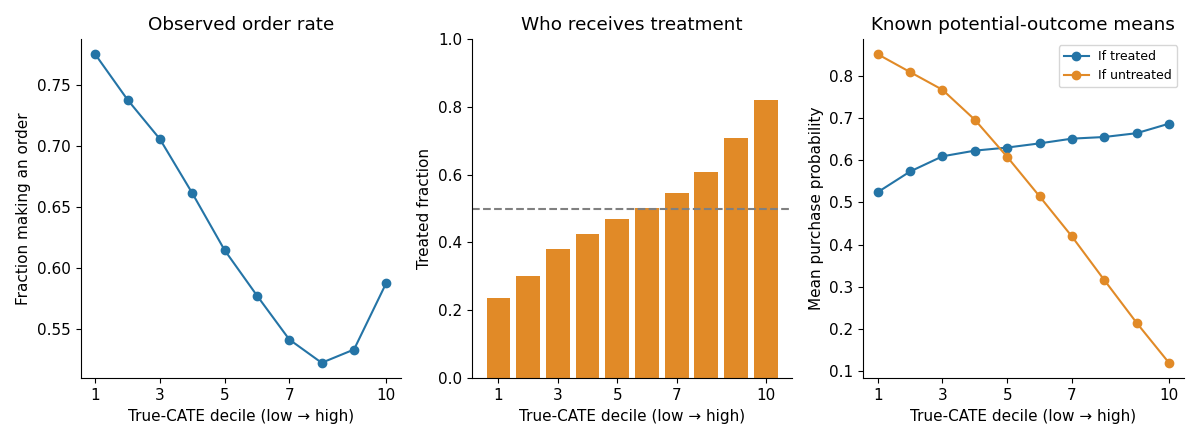
Figure 1: The customers are grouped by their true-CATE into deciles of approximately equal size. For each decile the assignment panel contains the 50/50 treatment budget, which did not lead to the equally sized customer profiles. Source: simulated data in this article. The figures have been created with Python.
We trained on 700k customers and then evaluated on the 300k held-out customers using seed 42 for this example. Each of the S, T, X, DA, DR, DML estimators were implemented using both linear and “boosted” base models. Note that all of the estimators above (S,T,X,DA,DR,DML) have lengthy derivations and are a material for another article. Here I will just provide the high-level intuition of the algorithms.
How its effect estimate is constructed
One outcome model; change the treatment flag and subtract predictions.
Separate treated and control outcome models; subtract predictions.
Regress imputed effects in each arm, then combine them.
Reweight outcome-model fitting across arms, then regress imputed effects.
Regress cross-fitted, doubly robust pseudo-outcomes.
Fit an effect function to cross-fitted treatment and outcome residuals.
The models used for this article are the EconML implementations (the S- and T-learners as well as the DA-, DR-, and DML-learners with a linear and XGBoost base model).
Our starting point will be an S-learner as the simplest and the most intuitive model. Its holdout MSE against the true CATE is 0.0006, with correlation 0.9964. That tells us its effect estimates are quite accurate in this simulation. But in reality we don’t know the true effect, so we need another way to assess targeting.
Looking at uplift without knowing the truth
The most obvious way to do this is an uplift barplot. We sort customers by the CATE, divide them into buckets and compare treatment and control outcomes for the buckets.
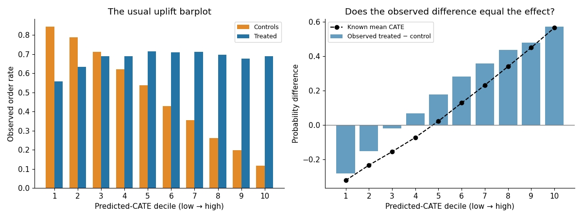
Figure 2. Left: the observed purchase rates in treated and control customers. Right: their difference, with the known mean CATE added as a simulation check. Both use the S-learner’s predicted-effect deciles. Source: this article’s simulated data, plotted with Python.
The graphs look useful: the right-hand buckets have larger observed differences than the left-hand ones. However, those differences are not quite the true effects. Grouping by predicted CATE does not necessarily make the treatment and control customers comparable inside each bucket — they can be very different in their characteristics
The plot helps us inspect a model, but we should not interpret its bar differences as causal effects or use only them to decide who should receive treatment.
Quite often we just need a single number, which allows us to compare different estimators. Something more or less similar to the ROC AUC score we sometimes use for classification model assessment. That’s where the Qini AUC comes to our attention.
From uplift bars to the Qini curve
Instead of having a barplot that compares uplift for a number of different buckets of customers, look at the single customer with the highest predicted value of treatment. Then add the next customer with the highest predicted value, then the next customer, and so on. For each customer added in the group we calculate the total positive outcomes for the treatment and control.
Rₜ(k) and R꜀(k) denote the positive-outcome totals for the treatment group and the control group, respectively, for the top k customers. Denote by Nₜ(k) and N꜀(k) the arm sizes for the treatment group and the control group. The Qini metric is then defined as:
Q(k)=Rt(k)−Rc(k)Nt(k)Nc(k).Q(k)=R_t(k)-R_c(k)\frac{N_t(k)}{N_c(k)}.Q(k)=Rt(k)−Rc(k)Nc(k)Nt(k).
Let p̂=Nₜ(N)/N be the observed treatment share in the evaluation sample. First define q(f)=Q(k)/(Np̂), where f=k/N, and let A_Q be its area above the line connecting the start and end points:
AQ=∫01[q(f)−fq(1)]df.A_Q=\int_0^1[q(f)-fq(1)]\,df.AQ=∫01[q(f)−fq(1)]df.
Zero is the reference area for random targeting; finite-sample scores can fluctuate around it. The normalization by N and horizontal fraction f=k/N are already included above, so we do not divide this area by N² again. Dividing by the treatment share supplies the causal-gain unit convention, but does not remove selection bias.
For the additional calibration, let r₀ denote the true-CATE ranking in the higher-selectivity, seed-42 holdout. We use DR as the reference score and calculate the fixed divisors:
cQ=AQ(r0)ADR(r0)=1.5445,c_Q=\frac{A_Q(r_0)}{A_{DR}(r_0)}=1.5445,cQ=ADR(r0)AQ(r0)=1.5445,
cIPW=AIPW(r0)ADR(r0)=1.0006.\qquad c_{IPW}=\frac{A_{IPW}(r_0)}{A_{DR}(r_0)}=1.0006.cIPW=ADR(r0)AIPW(r0)=1.0006.
All displayed evaluation areas and differences then use:
AQcal(r)=AQ(r)cQ,AIPWcal(r)=AIPW(r)cIPW,ADRcal(r)=ADR(r).A_Q^{cal}(r)=\frac{A_Q(r)}{c_Q}, \qquad A_{IPW}^{cal}(r)=\frac{A_{IPW}(r)}{c_{IPW}}, \qquad A_{DR}^{cal}(r)=A_{DR}(r).AQcal(r)=cQAQ(r),AIPWcal(r)=cIPWAIPW(r),ADRcal(r)=ADR(r).
All three reference scores therefore start as 0.0826. The curve below is also divided by c_Q, so its area matches the tables. This is an oracle-assisted calibration for this simulation: it requires knowing the true-CATE ranking and does not establish that the scores estimate the same quantity accurately. They are calibrated only for comparability purposes. The calibration preserves each evaluator’s model ordering. We freeze these constants everywhere, including within bootstrap resamples.
Numbers are rounded for display. Differences and confidence intervals are calculated before rounding, so equal displayed scores need not be identical.
Here is the S-learner’s Qini curve for the illustration:
Figure 3: Calibrated Qini for the fitted S-learner (solid line) and true-CATE ranking (dashed line). The dotted diagonal is the random-ranking baseline. Their areas above the diagonal are 0.0824 and 0.0826. The same fixed Qini divisor is used for both curves. Both scores still use observed treatments and outcomes, even when the order comes from true CATE. Source: Python simulation for this article.
The main problem is that the Qini metric in its evaluation still uses the observed treatments and outcome variables. Remember that the customers were selected for treatment based on their characteristics, thus the treatment/control differences still contain selection bias.
A causal learner estimates the treatment effect. If done correctly, it is potentially unconfounded. But the metric is still confounded, as it is observational! We’ve seen it already at the graph with the uplift bars — the difference was not matching the true effect.
This mismatch might be an insignificant calculation artifact if it wasn’t for its potential effect on qualitative conclusions based on the analysis. In our example, when we compare the models, Linear DR learner gives us better metrics than the “oracle” model, which knows the true CATE. This is indicative of a large problem. Now we know we can’t trust Qini, because it can choose a wrong estimator for us.
Therefore, we now understand, that we need to improve not just a learner, but the evaluation as well. The ideal situation of course — randomized treatment assignment. But when we have only biased observational data — we can use Inverse-Propensity Weighting (IPW) or Doubly Robust (DR) score which we discuss below.
Adjusting the evaluation with IPW and DR
Inverse-propensity weighting gives each observed outcome a weight based on how likely its assignment was:
ZiIPW=TiYie^(Xi)−(1−Ti)Yi1−e^(Xi).Z_i^{IPW}=\frac{T_iY_i}{\hat e(X_i)}-\frac{(1-T_i)Y_i}{1-\hat e(X_i)}.ZiIPW=e^(Xi)TiYi−1−e^(Xi)(1−Ti)Yi.
Doubly robust scoring also uses the outcome prediction and the residual, but weights the residual by the inverse propensity score of the customer.
ZiDR=μ^1(Xi)−μ^0(Xi)+Ti[Yi−μ^1(Xi)]e^(Xi)−(1−Ti)[Yi−μ^0(Xi)]1−e^(Xi).Z_i^{DR}=\hat\mu_1(X_i)-\hat\mu_0(X_i)+\frac{T_i[Y_i-\hat\mu_1(X_i)]}{\hat e(X_i)}-\frac{(1-T_i)[Y_i-\hat\mu_0(X_i)]}{1-\hat e(X_i)}.ZiDR=μ^1(Xi)−μ^0(Xi)+e^(Xi)Ti[Yi−μ^1(Xi)]−1−e^(Xi)(1−Ti)[Yi−μ^0(Xi)].
In the formulas above, T means the treatment flag, Y — the outcome variable. ê(X_i) — the propensity model (probability of being treated), μ̂₀(X_i) and μ̂₁(X_i) — the models of the outcome prediction under treatment and control.
Usually, the DR-learner uses the same pseudo-outcome as you see above to fit effects, but here we are not looking for it — we are evaluating a trained ranking. The ranking can come from any model — not just DR-learner.
Next step — we sort customers by the model ranked scores, summing up the corresponding scores:
G(f)=1N∑i∈topfNZi,AG=∫01[G(f)−fG(1)]df.G(f)=\frac1N\sum_{i\in\mathrm{top}\ fN} Z_i,\qquad A_G=\int_0^1[G(f)-fG(1)]\,df.G(f)=N1i∈topfN∑Zi,AG=∫01[G(f)−fG(1)]df.
These are the uncalibrated IPW and DR gain curves. IPW and DR adjust for confounding under their respective assumptions. Under randomized assignment, treatment-share-normalized Qini targets the same causal-gain convention. For display throughout this article, we additionally divide the IPW curve and area by the fixed reference divisor c_IPW; DR stays unchanged. Calibration is separate from the causal adjustment.
For the adjusted methods, we estimate a propensity model and two outcome models separately from the main ranking model. They are called the nuisance models. They are estimated using the observable variables X, T, and Y. For the nuisance models, we use three-fold crossfitting, which guarantees that for both predictions the customer was excluded from the training sample for the models. All rankings use the same evaluation scores.
Running the following Python code in the companion directory trains the S-learner and, in addition, fits separate evaluation models.
import numpy as npfrom sklearn.model_selection import train_test_splitfrom uplift_lib import ( generate_dataset, FEATURES, model_factories, crossfit_evaluation_nuisance, adjusted_scores, gain_curve, qini_auc, area,)data = generate_dataset(1_000_000, seed=42, assignment="selection_high")train, test = train_test_split( np.arange(len(data)), test_size=0.3, random_state=42)X = data[FEATURES].to_numpy()y = data.MadeOrder.to_numpy()t = data.TreatmentGroup.to_numpy()model = model_factories(family="xgb", seed=42, threads=4)["S"]()model.fit(y[train], t[train], X=X[train])ranking = model.effect(X[test]).ravel()evaluation = data.iloc[test].reset_index(drop=True)observed = evaluation[FEATURES + ["TreatmentGroup", "MadeOrder"]]nu, audit = crossfit_evaluation_nuisance(observed, seed=2042)ipw = adjusted_scores( evaluation.MadeOrder, evaluation.TreatmentGroup, nu.e_hat)dr = adjusted_scores( evaluation.MadeOrder, evaluation.TreatmentGroup, nu.e_hat, nu.mu0_hat, nu.mu1_hat,)c_q = 1.5445466434481507 # Frozen high-policy seed-42 reference.c_ipw = 1.0005932054691182print( "Calibrated Qini", qini_auc(evaluation.MadeOrder, evaluation.TreatmentGroup, ranking) / evaluation.TreatmentGroup.mean() / c_q,)print("Calibrated IPW", area(*gain_curve(ranking, ipw)) / c_ipw)print("DR", area(*gain_curve(ranking, dr)))
The errors in the evaluation of different estimators are close to each other, so we better look at the error of the score of each ranking with respect to the causal gain of that ranking, which is known from the data generation process (thanks to our synthetic dataset!).
Figure 4: Calibrated evaluator score minus known causal gain for each boosted learner’s ranking. All three evaluators are shown together on one common axis. The reference true-CATE scores have been matched by construction; these points show the remaining disagreement for other rankings. Positive values mean overstatement; negative values mean understatement. These are signed errors, not absolute errors. Source: this article’s simulated data, plotted with Python.
After calibration, Qini’s residual errors across the six boosted rankings range from +0.0002 to +0.0008. Calibrated IPW errors range from +0.0001 to +0.0002, and DR errors from +0.0001 to +0.0002. Qini favors the wrong ranking in the Linear-DR comparison below.
The disagreement matters for model choice, too:
The “true gain” is the area above the endpoint diagonal of the cumulative true-CATE curve for each ranking. IPW and DR produce scores close to these known gains and favor the true-CATE ranking over Linear DR. They do not reproduce every small ordering difference among the boosted learners. Calibrated Qini still favors Linear DR over the true-CATE ranking.
When you use these methods — keep in mind that IPW still requires a correct propensity model, and DR still requires a correct propensity OR both outcome models. Both scorers require consistency, no unmeasured confounding and overlap. Estimated models and finite samples leave residual error, so these approaches are not automatically unbiased scores for every dataset. So, you use it, but be careful as always.
Are the differences between models convincing?
We have only compared point estimates for the different models so far. It might be interesting to see how large the differences are between the estimates for another random set of evaluation customers (i.e. different realization of the holdout sample of 300k customers with their respective multiplicities). In other words — are these differences statistically significant and consistent?
In order to investigate this we conducted 1,000 paired bootstrap resamples of the 300,000 customers in the holdout data set. For each of the resampled evaluation data sets, we computed the statistics of interest for all models and all evaluation methods. The resulting values’ 2.5th and 97.5th percentiles are provided in brackets below.
These are the conditional 95% percentile intervals. Note that we hold the trained models and nuisance functions fixed and resample only the evaluation part. This means we don’t guarantee the 95% coverage for the full procedure bootstrap. The experiment is repeated later with 3 different seeds to ensure the conclusions are robust.
Calibrated Qini and conditional 95% interval
DR gain and conditional 95% interval
The models use the same data seed. Qini’s treatment-share denominator is recomputed within each bootstrap resample, then the fixed calibration divisor is applied. Fits and calibration constants remain fixed, so intervals exclude calibration-estimation uncertainty. Reference point estimates coincide by construction; their intervals need not coincide. The IPW interval is omitted for simplicity.
Note that overlapping intervals do not directly answer questions of whether one model is better than another. More relevant are the intervals for the paired differences between the two models under consideration (how much one model is better than another). Below we compared each of the models with the oracle truth.
Figure 5. Each point is the model’s score minus the true-CATE ranking’s score, with a paired conditional 95% interval. Positive values favor the model; negative values favor true CATE. Left: calibrated Qini. Right: DR gain. The reference scores coincide; horizontal axis limits differ for readability. Calibration constants remain fixed across resamples. All seven DR-gain intervals lie below zero (as expected), while Qini favors Linear DR, XGBoost DR and XGBoost DML over true CATE. The models and nuisance fits are held fixed, and intervals are unadjusted for multiple comparisons. Source: this article’s simulated data, plotted with Python.
Which estimator would we choose here?
Choosing a CATE estimator is a broader topic that deserves a separate article. For this example, I would choose the XGBoost S-learner as a simple starting point. It has the simplest estimation structure among the six learners considered: one outcome model, with treatment included as an input feature. The DML estimator has the highest DR-gain point estimate among the six boosted learners, but its advantage over S is small: the paired S-minus-DML difference is -0.00006, with a conditional 95% interval which includes zero. That does not prove equivalence and this is not the claim that S learner is always the best. But if the difference in the 5th digit is not critical for your application, I would choose the S-learner for this specific case. Simplicity wins.
Positive differences favor S; negative differences favor the other learner. Intervals use 1,000 paired evaluation-row resamples with ranking models and nuisance fits held fixed and are unadjusted for multiple comparisons. Source: this article’s simulated data, plotted with Python.
Conditional 95% interval
The comparison of S with T has a positive DR-area difference of +0.0002 with a Conditional 95% Interval of [+0.00003, +0.0003]. So, within these models and this fixed set of nuisance fits, S has a statistically significant DR-area difference compared with T. The paired intervals for the comparisons with X, DA, DR, and DML all include zero, so there is no evidence of a consistently higher DR area for S.
We don’t use Qini here anymore, because we’ve seen before that its confoundedness affects its conclusions even on a qualitative scale. Even increasing bootstrap sample for the Qini won’t make it unbiased, so we can stop using it.
Does the assignment policy change the result
We have so far followed one data generation to model comparison example. Let’s now slightly change the assignment policy and check if the results are stable under different assignments.
We will replace 2.5 in the propensity rule by 0.5 and by 1, affecting the selection bias and we will call it “low” and “middle” selectivity. The population treatment share will still be 50% as we have calibrated our assignment in this way. We will also refit all the learners for 3 different seeds for robustness.
For this figure, we rank customers directly by their known true CATE. No S, T or other learner supplies the ranking. We hold the customer profiles and this perfect ordering fixed across assignment policies within each seed, then change which customers receive treatment and which outcomes we observe. The question is whether each evaluator can accurately score the same ranking as assignment becomes more selective.
All three evaluators’ point estimates will coincide in the “higher” selection policy by construction because of the calibration we’ve done for comparability. The calibration is made based on the true CATE and we are considering the true CATE ranking in this case. What is interesting is how the rankers behave in case of the changes in the assignment policy.
We see that the DR and IPW behave quite stable, and the Qini is not stable at all and changing a lot depending on the assignment policy. This is one more evidence of how it can be influenced by different levels of selection bias.
Figure 6. Calibrated evaluator score minus known causal area for the same true-CATE ranking. Left: all evaluators. Right: calibrated IPW and DR on an expanded scale. Calibration constants are fixed from the higher-selectivity, seed-42 reference; they are not recalculated for each policy or seed. Dots show means over three seeds; whiskers show minimum to maximum, not confidence intervals. Source: this article’s simulated data, plotted with Python.
All three runs of increased selectivity show the same reversal between Linear DR and true CATE as was seen in the single run of increased selectivity. The expected-count diagnostic is also well-behaved. This constitutes more empirical evidence for the phenomenon than a single lucky or unlucky run. (Of course, three runs do not guarantee to cover the variability in all possible datasets.)
Does a small amount of tuning change the comparison?
What about hyperparameter tuning? The evaluator also affects which hyperparameters we select! We gave each of the six boosted learners 15 configurations, including its default. The original 700,000 training customers were split into 500,000 for fitting candidates and 200,000 for validation. Then we selected each learner’s configuration using cross-fitted DR gain on that validation sample, without using true CATE.
Then we have frozen the selected hyperparameters before generating a fresh 300,000-customer test sample from the "high" selectivity policy. Both default and selected models were refitted on the same original 700,000 training customers, then evaluated on these new test customers with shared cross-fitted evaluation models. The earlier article holdout was not used in this tuning comparison. So, do not attribute differences from earlier tables to tuning alone. Below you will see the illustrated effect of the tuning on the three metrics considered before and on the RMSE metric which is calculated relative to the true CATE which we know as we have generated our dataset (it’s omitted from other sections, because in reality we never know the true CATE).
Figure 7. The plot shows the ranking and customer profiles for the six learners, evaluated on a fresh sample of 300,000 customers. The evaluator panels use calibrated Qini, calibrated IPW and unchanged DR, with the same fixed reference constants as the earlier tables. Qini remains confounded; IPW and DR rely on their causal assumptions. We also plot the CATE RMSE here against the synthetic known ground-truth. The vertical axes of the sub-panels have been expanded to make it possible to see the small differences between the DR evaluation before and after tuning for each learner. The panels have otherwise different scales. Source: this article’s simulated data, plotted with Python.
Paired conditional 95% interval
Figure 8: 1,000 paired row-bootstrap resamples on the fresh test sample. Positive values favor the tuned version of the model. All intervals condition on the ranking and the fit of the evaluation model. The intervals do not include the variability introduced by the hyperparameter search and retraining of the models for the comparison. Source: simulated data from the article for this test case. Figure plotted with Python.
The direction of the effect from our tuning is not clear for S, X, DA, DR, and DML learners as the intervals include zero, which corresponds to no change in the values. But for T-learner the paired intervals all favor tuning which also improves the CATE RMSE from 0.0328 to 0.0237. S-learner has the most extreme behavior where the DR point estimate decreased, and the CATE RMSE increased from 0.0243 to 0.0316 on the fresh test sample. So our tuning in case of the S-learner was not very fruitful.
To be clear, it’s still hard to compare the tuning of such different models, as the number of potential hyperparameter changes is different for a simple S-learner and for the DML. But the idea of this section is to show that the hyperparameter tuning doesn’t change the ranking effect of confounded metric (Qini) we’ve shown before.
What to do when comparing uplift models
In conclusion, let’s try to formulate — what should we do when comparing the uplift models quality? First evaluate the assignment to treatment in your experiment. If the assignment to treatment is not random (as in most cases) then a familiar uplift plot or Qini curve don’t work anymore. Use both an evaluation design and the estimator which assumptions still hold (don’t require random assignment).
Using IPW and a DR evaluator of causal gain on the data gave scores close to the known causal gain and kept the estimators ranking correct. I would opt for the DR evaluation, well, because it’s Doubly Robust, so it’s still valid even if one of its assumptions failed.
Ultimately, for your marketing campaign (or any other application of the uplift model) look at what’s important for your case: the budget, cost and incremental value for a given budget. Area under the curve is interesting but not what you are optimizing for as the business objective.
Code and reproducibility
The separate evaluation companion contains evaluation.ipynb, the shared model and metric implementation, all numerical tables, paired bootstrap draws, figures and the tuning protocol. Its default notebook run analyzes the completed experiments and independently checks IPW/DR formulas from stored observed rows and nuisance predictions.
python reproduce.py --output regenerated recreates all baseline fits, evaluator fits, diagnostics, resamples, tuning and figures in a new directory. The single code example above is supplied as article_example.py. The README distinguishes these full fitting steps from quick notebook analysis. Three-policy seed ranges and fixed-fit bootstrap intervals retain their separate meanings.
[1] PyWhy, EconML Meta-Learners, version 0.16.0 documentation.
[2] E. H. Kennedy, Towards optimal doubly robust estimation of heterogeneous causal effects (2020; revised 2023), arXiv.
[3] scikit-uplift contributors, Metric implementation, version 0.5.1 documentation.
[4] grf contributors, Assessing heterogeneity with RATE, documentation. Our own conditional row-bootstrap procedure is used in this article instead of grf’s implementation of RATE for causal heterogeneity inference.
Machine Learning can be easy and intuitive - here's a complete from-scratch guide to Decision Trees.
April 8, 202110 min read
Leveraging LangChain to move from ad-hoc Jupyter Notebooks to production modular service
October 30, 202323 min read
Configuring GPU libraries on Ubuntu 20.4 LTS
December 31, 20206 min read
Two Neural Network Regression Problems
February 13, 20204 min read
A stance on the opportunity for out-of-the-box insight for standard schemas
October 23, 202011 min read
A Visual Atlas of Popular Culture
December 31, 20217 min read
An easy-to-follow tutorial for Vim text editor
March 6, 202311 min read
A simple mathematical intuition behind one of the commonly used optimisation algorithms in Machine Learning.
March 18, 20199 min read
This article is a comprehensive overview of using Transformers for automatic topic discovery
January 26, 20226 min read
原文为英文,正文由自动抓取并保留原文。
原文发布于 Towards Data Science(When Qini Rewards the Wrong Uplift Model, Use Doubly Robust Scores),标题、摘要与正文由机器翻译,术语按行业惯例统一,未经人工逐句校订。