在 PyTorch 中计算量子机器学习模型的有效维度

本文由 Jacob L. Cybulski 联合撰写。
我们究竟该如何实现有效维度?
本文是关于将有效维度理解为量子模型学习能力度量的两部分系列文章的第二部分。在第一篇文章中,我们建立了有效维度背后的直觉,并讨论了为什么单纯统计原始参数量并不能告诉我们一个模型真正有多复杂。第一部分聚焦于这一度量的理论层面,而本文则逐步讲解其在 PyTorch 中的实现。
有效维度源自数学与信息论中的统计复杂性度量,随后被改造用于量化经典机器学习和量子机器学习中的模型容量与表达能力——以及后来的可训练性 [1, 2]。其核心在于,这一度量回答了一个直白的问题:我们的模型中有多少个参数方向是数据真正能够区分的?
当我们审视有效维度的数学公式(已在第 1 部分中解释过)时,两个实际挑战立刻显现:
我们如何估计任意模型的 Fisher 信息矩阵?
我们如何计算模型参数空间上的积分?
这两个挑战听起来可能令人生畏,但它们都有简洁而实用的解决方案。在本指南中,我们将拆解这两个挑战,并展示如何在代码中可靠地计算有效维度。
估计 Fisher 信息矩阵
在计算有效维度之前,我们需要估计 Fisher 信息矩阵(FIM)。我们会针对选定的参数向量 θ 和给定的输入样本 x 计算该矩阵。
为了具体说明其机制,考虑一个参数化量子电路。模拟时,该电路会返回一个量子态向量:
\ket{\psi(\boldsymbol{x}, \boldsymbol{\theta})}. \tag{1}∣ψ(x,θ)⟩.(1)
在计算基中测量到结果 y 的概率由振幅的模平方给出:
p(y \mid \boldsymbol{x}; \boldsymbol{\theta}) = \left|\braket{y \mid {\psi(\boldsymbol{x}, \boldsymbol{\theta})}}\right|^2. \tag{2}p(y∣x;θ)=∣⟨y∣ψ(x,θ)⟩∣2.(2)
对于每个概率不可忽略的测量结果,我们使用 PyTorch 的自动微分(autograd)来计算概率相对于电路参数的梯度:
(\frac{\partial}{\partial\theta_1}p(y \mid \boldsymbol{x}; \boldsymbol{\theta}), \frac{\partial}{\partial\theta_2}p(y \mid \boldsymbol{x}; \boldsymbol{\theta}),\dots, \frac{\partial}{\partial\theta_k}p(y \mid \boldsymbol{x}; \boldsymbol{\theta})), \tag{3}(∂∂θ1∂p(y∣x;θ),∂θ2∂p(y∣x;θ),…,∂θk∂p(y∣x;θ)),(3)
其中 kkk 是模型的参数数量。理论上,(i,j)(i,j)(i,j) 元素的 Fisher 信息矩阵被定义为对所有可能输入和输出的期望值:
F(i,j)(θ)=E[(∂∂θilogp(x,y;θ))(∂∂θjlogp(x,y;θ)|θ].(4) \boldsymbol{F}_{(i,j)}(\boldsymbol{\theta}) = \mathbb{E} \left[ \left(\frac{\partial}{\partial\theta_i} \log p(\boldsymbol{x},{y};\boldsymbol{\theta})\right) \left(\frac{\partial}{\partial\theta_j} \log p(\boldsymbol{x},{y};\boldsymbol{\theta})\right) \middle| \,\boldsymbol{\theta} \right]. \tag{4}F(i,j)(θ)=E[(∂θi∂logp(x,y;θ))(∂θj∂logp(x,y;θ))
对于几乎所有现实世界中的模型,这一期望都没有闭式解。我们无法在整个数据分布上评估所有可能的结果。相反,我们通过对一批具有代表性的 ℓ 个数据样本取平均来近似它。这给出了经验 Fisher 信息矩阵:
F~(i,j)(θ):=1ℓ∑m=1ℓ(∂∂θilogp(xm,ym;θ))(∂∂θjlogp(xm,ym;θ)).(5) \tilde{\boldsymbol{F}}_{(i,j)}(\boldsymbol{\theta}) := \frac{1}{\ell} \sum_{m=1}^\ell \left(\frac{\partial}{\partial\theta_i} \log p(\boldsymbol{x}_m,{y}_m;\boldsymbol{\theta}) \right) \left( \frac{\partial}{\partial\theta_j} \log p(\boldsymbol{x}_m,{y}_m;\boldsymbol{\theta}) \right). \tag{5}F~(i,j)(θ):=ℓ1m=1∑ℓ(∂θi∂logp(xm,ym;θ))(∂θj∂logp(xm,ym;θ)).(5)
利用恒等式 ∂∂θilogp=1p∂p∂θi\frac{\partial}{\partial\theta_i} \log p = \frac{1}{p}\frac{\partial p}{\partial\theta_i}∂θi∂logp=p1∂θi∂p,其中概率的参数被隐式保留,外积变为:
(∂∂θilogp)⋅(∂∂θjlogp)=1p2∂p∂θi∂p∂θj.(6) \left( \frac{\partial}{\partial\theta_i} \log p \right) \, \cdot \left(\frac{\partial}{\partial\theta_j} \log p\right) = \frac{1}{p^2}\frac{\partial p}{\partial\theta_i} \, \frac{\partial p}{\partial\theta_j}. \tag{6}(∂θi∂logp)⋅(∂θj∂logp)=p21∂θi∂p∂θj∂p.(6)
当以结果概率 ppp 加权时,分母恰好约简为 ppp。
在实践中,如果一个结果的概率接近零,除以 ppp 可能导致数值误差。为了防止除以零,我们引入一个小阈值(min_probability),跳过可忽略的结果。
以下函数展示了如何在 PyTorch 中针对给定输入估计 Fisher 矩阵:
weights = net.qlayers.weightsflat_weights = weights.reshape(-1)k_params = flat_weights.numel()# Get model output probabilitiesstate = net.state_circuit(inputs, weights)probabilities = torch.abs(state) ** 2probabilities = probabilities.reshape(-1)fisher = torch.zeros( (k_params, k_params), dtype=weights.dtype, device=weights.device,)for probability in probabilities: if probability.detach() > min_probability: gradient = torch.autograd.grad( probability, weights, retain_graph=True, )[0].reshape(-1) fisher += torch.outer(gradient, gradient) / probability
参数采样:求解积分
有效维度的公式涉及在参数空间 Θ\ThetaΘ 上的积分。对于全局有效维度,我们在整个参数空间上积分。对于局部有效维度,我们仅在一个以感兴趣特定点(例如我们训练好的权重)为中心、半径为 ε\varepsilonε 的球体内积分。
由于该积分无法解析求解,我们使用蒙特卡洛方法。蒙特卡洛积分背后的思想很直接:
从参数空间中随机且均匀地采样点。
在每个采样点处计算函数值。
将结果取平均。
随着随机样本数量的增加,样本平均值会收敛到积分的真实体积平均值。这样可以避免直接计算复杂的积分。
为全局有效维度进行采样
在参数化量子电路中,门参数是态旋转角,天然限制在 000 和 2π2\pi2π 之间。为了计算全局有效维度,我们只需从该区间独立且均匀地采样每个参数:
θi∼U(0,2π).(7)\theta_i \sim \mathcal{U}(0, 2\pi). \tag{7}θi∼U(0,2π).(7)
我们可以用一个简单的辅助类来实现这个均匀参数采样器:
class UniformParameterSpace: def __init__(self, low, high, shape, dtype=torch.float32, device="cpu"): self.low = low self.high = high self.shape = shape self.dtype = dtype self.device = device def sample(self): return torch.empty( self.shape, dtype=self.dtype, device=self.device ).uniform_(self.low, self.high)
局部有效维度采样:为何朴素采样会失败
对于局部有效维度,我们希望从以参考参数向量 θ∗ 为中心、半径为 ε 的球(ε-球)中均匀采样。
乍一看,从圆形或球体中均匀采样似乎很简单。在二维极坐标中,一个点由到中心的距离 r 和角度 φ 定义。人们很容易写出:
r∼U(0,ε) 且 φ∼U(0,2π)。(8)
然而,这种朴素方法会失败。如果我们用这种方式采样 10,000 个点并绘制它们的位置,会看到大量点密集地聚集在中心附近,而外缘则很稀疏(见图 1)。
图 1。对 r 和 φ 进行均匀采样并不会在圆盘上产生均匀采样。点明显集中在中心,使外部区域覆盖稀疏。图片由作者提供。
图 1 表明,对半径 r 和角度 φ 进行均匀采样并不会在圆盘上产生均匀分布。左图显示了单位圆盘上得到的点,中心附近明显聚集。右图通过绘制估计密度 N(R)/(πR²) 随圆盘半径 R 的变化来量化这一效应。随着 R 增大,密度迅速下降,证实外部区域比中心覆盖得更稀疏。
为了理解这个问题,可以想象把圆盘划分成若干径向宽度相等的细圆环。由于 rrr 是均匀采样的,每个圆环都对应相同的区间 Δr\Delta rΔr,因此获得相同的概率质量。我们用 ΔP\Delta PΔP 表示这个相同的概率质量。换句话说,ΔP\Delta PΔP 是一个采样点落在某个特定径向圆环内的概率。
原文较长,译文为节选;译文由英文原文机器翻译,术语按行业惯例统一,可在文末展开原文核对。
查看英文原文(Computing Effective Dimension for Quantum ML Models in PyTorch)
This article was co-authored by Jacob L. Cybulski.
How Can We Actually Implement Effective Dimension?
This article is the second part of a two-part series on understanding effective dimension as a measure of a quantum model's learning capacity. In the first article, we built the intuition behind effective dimension and discussed why counting raw parameters does not tell us how complex a model truly is. While the first part focused on the theoretical aspect of this measure, this article explains its implementation step by step in PyTorch.
Effective dimension emerged from statistical complexity measures in mathematics and information theory, and was subsequently adapted to quantify model capacity and expressiveness—and later trainability—in classical and quantum machine learning [1, 2]. At its core, the metric answers a straightforward question: how many parameter directions in our model can the data actually distinguish?
When we look at the mathematical formula for effective dimension (previously explained in Part 1), two practical challenges immediately stand out:
How do we estimate the Fisher information matrix for an arbitrary model?
How do we compute an integral over the model's parameter space?
Both challenges can sound intimidating, but they have clean and practical solutions. In this guide, we will break down both challenges and show how to compute effective dimension reliably in code.
Estimating the Fisher Information Matrix
Before calculating effective dimension, we need to estimate the Fisher Information Matrix (FIM). We compute this matrix for a chosen parameter vector θ\boldsymbol{\theta}θ and a given input sample x\boldsymbol{x}x.
To illustrate the mechanics concretely, consider a parameterized quantum circuit. When simulated, the circuit returns a quantum state vector:
∣ψ(x,θ)⟩.(1)\ket{\psi(\boldsymbol{x}, \boldsymbol{\theta})}. \tag{1}∣ψ(x,θ)⟩.(1)
The probability of measuring an outcome yyy in the computational basis is given by the squared magnitude of the amplitude:
p(y∣x;θ)=∣⟨y∣ψ(x,θ)⟩∣2.(2) p(y \mid \boldsymbol{x}; \boldsymbol{\theta}) = \left|\braket{y \mid {\psi(\boldsymbol{x}, \boldsymbol{\theta})}}\right|^2. \tag{2}p(y∣x;θ)=∣⟨y∣ψ(x,θ)⟩∣2.(2)
For each measurement outcome with non-negligible probability, we use PyTorch's automatic differentiation (autograd) to calculate the gradient of the probability with respect to the circuit parameters:
(∂∂θ1p(y∣x;θ),∂∂θ2p(y∣x;θ),…,∂∂θkp(y∣x;θ)),(3) \left( \frac{\partial}{\partial\theta_1}p(y \mid \boldsymbol{x}; \boldsymbol{\theta}), \frac{\partial}{\partial\theta_2}p(y \mid \boldsymbol{x}; \boldsymbol{\theta}),\dots, \frac{\partial}{\partial\theta_k}p(y \mid \boldsymbol{x}; \boldsymbol{\theta})\right), \tag{3}(∂θ1∂p(y∣x;θ),∂θ2∂p(y∣x;θ),…,∂θk∂p(y∣x;θ)),(3)
with kkk being the number of parameters of the model. In theory, the Fisher information matrix for the (i,j)(i,j)(i,j) element is defined as an expectation value over all possible inputs and outcomes:
F(i,j)(θ)=E[(∂∂θilogp(x,y;θ))(∂∂θjlogp(x,y;θ))|θ].(4) \boldsymbol{F}_{(i,j)}(\boldsymbol{\theta}) = \mathbb{E} \left[ \left(\frac{\partial}{\partial\theta_i} \log p(\boldsymbol{x},{y};\boldsymbol{\theta})\right) \left(\frac{\partial}{\partial\theta_j} \log p(\boldsymbol{x},{y};\boldsymbol{\theta})\right) \middle| \,\boldsymbol{\theta} \right]. \tag{4}F(i,j)(θ)=E[(∂θi∂logp(x,y;θ))(∂θj∂logp(x,y;θ))
For almost any real-world model, this expectation has no closed form. We cannot evaluate every possible outcome over the entire data distribution. Instead, we approximate it by averaging over a representative batch of ℓ\ellℓ data samples. This gives the empirical Fisher information matrix:
F~(i,j)(θ):=1ℓ∑m=1ℓ(∂∂θilogp(xm,ym;θ))(∂∂θjlogp(xm,ym;θ)).(5) \tilde{\boldsymbol{F}}_{(i,j)}(\boldsymbol{\theta}) := \frac{1}{\ell} \sum_{m=1}^\ell \left(\frac{\partial}{\partial\theta_i} \log p(\boldsymbol{x}_m,{y}_m;\boldsymbol{\theta}) \right) \left( \frac{\partial}{\partial\theta_j} \log p(\boldsymbol{x}_m,{y}_m;\boldsymbol{\theta}) \right). \tag{5}F~(i,j)(θ):=ℓ1m=1∑ℓ(∂θi∂logp(xm,ym;θ))(∂θj∂logp(xm,ym;θ)).(5)
Using the identity ∂∂θilogp=1p∂p∂θi\frac{\partial}{\partial\theta_i} \log p = \frac{1}{p}\frac{\partial p}{\partial\theta_i}∂θi∂logp=p1∂θi∂p, where the arguments are kept implicit for the probabilities, the outer product becomes:
(∂∂θilogp)⋅(∂∂θjlogp)=1p2∂p∂θi∂p∂θj.(6) \left( \frac{\partial}{\partial\theta_i} \log p \right) \, \cdot \left(\frac{\partial}{\partial\theta_j} \log p\right) = \frac{1}{p^2}\frac{\partial p}{\partial\theta_i} \, \frac{\partial p}{\partial\theta_j}. \tag{6}(∂θi∂logp)⋅(∂θj∂logp)=p21∂θi∂p∂θj∂p.(6)
When weighted by the outcome probability ppp, the denominator cancels cleanly to ppp.
In practice, if an outcome has a probability near zero, dividing by ppp can cause numerical errors. To prevent division by zero, we introduce a small threshold (min_probability) that skips negligible outcomes.
The following function shows how to estimate the Fisher matrix for a given input in PyTorch:
weights = net.qlayers.weightsflat_weights = weights.reshape(-1)k_params = flat_weights.numel()# Get model output probabilitiesstate = net.state_circuit(inputs, weights)probabilities = torch.abs(state) ** 2probabilities = probabilities.reshape(-1)fisher = torch.zeros( (k_params, k_params), dtype=weights.dtype, device=weights.device,)for probability in probabilities: if probability.detach() > min_probability: gradient = torch.autograd.grad( probability, weights, retain_graph=True, )[0].reshape(-1) fisher += torch.outer(gradient, gradient) / probability
Parameter Sampling: Solving the Integral
The formula for effective dimension involves an integral over the parameter space Θ\ThetaΘ. For the global effective dimension, we integrate over the entire parameter space. For the local effective dimension, we only integrate over a ball of radius ε\varepsilonε around a specific point of interest (such as our trained weights).
Because this integral cannot be solved analytically, we use the Monte Carlo method. The idea behind Monte Carlo integration is straightforward:
Sample points randomly and uniformly from the parameter space.
Evaluate the function at each sampled point.
Average the results together.
As we increase the number of random samples, the sample average converges to the true volume average of the integral. This avoids having to compute a complex integral directly.
Sampling for Global Effective Dimension
In parameterized quantum circuits, gate parameters are state rotation angles naturally bounded between 000 and 2π2\pi2π. To evaluate the global effective dimension, we simply sample each parameter independently and uniformly from this interval:
θi∼U(0,2π).(7)\theta_i \sim \mathcal{U}(0, 2\pi). \tag{7}θi∼U(0,2π).(7)
We can implement this uniform parameter sampler with a simple helper class:
class UniformParameterSpace: def __init__(self, low, high, shape, dtype=torch.float32, device="cpu"): self.low = low self.high = high self.shape = shape self.dtype = dtype self.device = device def sample(self): return torch.empty( self.shape, dtype=self.dtype, device=self.device ).uniform_(self.low, self.high)
Sampling for Local Effective Dimension: Why Naive Sampling Fails
For the local effective dimension, we want to sample uniformly from a ball of radius ε\varepsilonε (ε\varepsilonε-ball) centered at a reference parameter vector θ∗\theta^*θ∗.
At first glance, sampling uniformly from a circle or ball seems simple. In 2D polar coordinates, a point is defined by its distance rrr from the center and its angle ϕ\phiϕ. It is tempting to write:
r∼U(0,ε)andϕ∼U(0,2π).(8) r \sim \mathcal{U}(0, \varepsilon) \quad \text{and} \quad \phi \sim \mathcal{U}(0, 2\pi). \tag{8}r∼U(0,ε)andϕ∼U(0,2π).(8)
However, this naive approach fails. If we sample 10,000 points this way and plot their locations, we see a heavy concentration of points clustered tightly near the center, while the outer edge is sparse (see Figure 1).
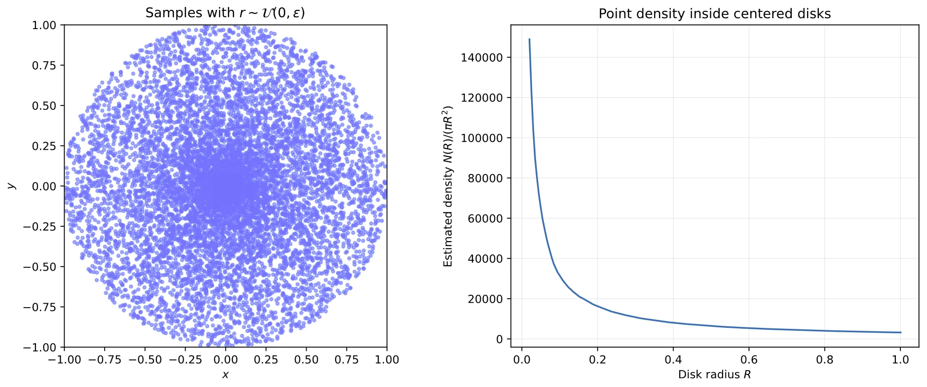
Figure 1. Uniform sampling of rrr and ϕ\phiϕ does not produce uniform sampling over a disk. Points visibly concentrate in the center, leaving outer regions sparsely covered. Image by authors.
Figure 1 shows that sampling the radius r and the angle φ uniformly does not yield a uniform distribution over a disk. The left panel displays the resulting points on the unit disk, with a visible concentration near the center. The right panel quantifies this effect by plotting the estimated density N(R)/(πR²) against the disk radius R. The density decreases rapidly as R grows, confirming that outer regions are covered more sparsely than the center.
To understand the problem, imagine splitting the disk into thin circular bands of equal radial width. Because rrr is sampled uniformly, each band corresponds to the same interval Δr\Delta rΔr and therefore receives the same probability mass. We denote this equal probability mass by ΔP\Delta PΔP. In other words, ΔP\Delta PΔP is the probability that one sampled point falls inside a particular radial band.
Figure 2 explains why this produces non-uniform sampling. Every radial band receives the same probability mass ΔP\Delta PΔP, because all bands have the same width Δr\Delta rΔr and rr r is sampled uniformly. However, an outer circular band has a much larger area than an inner band of the same width (A4≫A1A_4 \gg A_1A4≫A1).
Figure 2. This diagram showcases why sampling uniformly in rrr and ϕ\phiϕ does not produce uniform sampling from a disk. While having equal probability mass ΔP\Delta PΔP, the outermost surface is much larger (A4≫A1)(A_4 \gg A_1)(A4≫A1), therefore ρ1≫ρ4\rho_1 \gg \rho_4ρ1≫ρ4. Image by authors.
Figure 2 explains why sampling the radius and angle uniformly does not produce uniform sampling over a disk. The diagram highlights two cells with the same radial width Δr and angular width Δθ, and therefore the same probability mass ΔP. The innermost cell S1 has area A1, while the outermost cell S4 has area 7A1. Because the same probability mass is spread over a much larger area in the outer cell, the point density there is far lower, so ρ1 is much greater than ρ4.
As a result, the same expected number of sampled points is spread over a much larger area in the outer band. The point density is therefore
ρi=ΔPAi.(9)\rho_i = \frac{\Delta P}{A_i}. \tag{9}ρi=AiΔP.(9)
Since A4≫A1A_4 \gg A_1A4≫A1, we obtain
ρ1≫ρ4.(10)\rho_1 \gg \rho_4. \tag{10}ρ1≫ρ4.(10)
In short, uniform sampling in the radius gives every radial band equal probability, not every equal-area region equal probability. This is why the points cluster near the center of the disk.
To evenly distribute the points across the entire volume in kkk dimensions, we need to pull more points toward the outer shells. We do this by scaling the radius with a root of the dimension:
Pick a random direction u\boldsymbol{u}u on the unit sphere by sampling from a standard normal distribution and normalizing its length:
u=z∥z∥2,z∼N(0,I).(11) \boldsymbol{u} = \frac{\boldsymbol{z}}{\|\boldsymbol{z}\|_2}, \quad \boldsymbol{z} \sim \mathcal{N}(0, \boldsymbol{I}). \tag{11}u=∥z∥2z,z∼N(0,I).(11)
Scale the radius using a uniform random variable q∼U(0,1)q \sim \mathcal{U}(0, 1)q∼U(0,1):
r=εq1/k.(12)r = \varepsilon \, q^{1/k}. \tag{12}r=εq1/k.(12)
Shift the point to center it at θ∗\boldsymbol{\theta}^*θ∗:
θ=θ∗+ru.(13)\boldsymbol{\theta} = \boldsymbol{\theta}^* + r \boldsymbol{u}. \tag{13}θ=θ∗+ru.(13)
The exponent 1/k1/k1/k compensates exactly for the rapid volume growth of higher-dimensional spheres, ensuring that every region inside the ball has the same point density.
Here is the complete implementation of the ε\varepsilonε-ball sampler:
class EpsilonBallParameterSpace: def __init__(self, center, epsilon, generator=None): if epsilon <= 0: raise ValueError("epsilon must be positive") self.center = center.detach().clone() self.epsilon = epsilon self.generator = generator self.dimension = self.center.numel() def sample(self): # 1. Random direction on the unit sphere direction = torch.randn( self.dimension, dtype=self.center.dtype, device=self.center.device, generator=self.generator, ) direction = direction / torch.linalg.vector_norm(direction) # 2. Scale radius by q^(1/d) to achieve uniform volume density radius = self.epsilon * torch.rand( (), dtype=self.center.dtype, device=self.center.device, generator=self.generator, ).pow(1.0 / self.dimension) return (self.center.reshape(-1) + radius * direction).reshape_as(self.center)
Putting It Together: Stable Computation
Now that we can sample parameters and compute Fisher matrices, we can evaluate the effective dimension.
First, we estimate the empirical Fisher matrix for each sampled parameter configuration θi\boldsymbol{\theta}_iθi by averaging across our input dataset {xj}\{\boldsymbol{x}_j\}{xj} of size NxN_xNx:
F~(θi)=1Nx∑j=1NxF(θi,xj).(14)\tilde{\boldsymbol{F}}(\boldsymbol{\theta}_i) = \frac{1}{N_x} \sum_{j=1}^{N_x} \boldsymbol{F}(\boldsymbol{\theta}_i, \boldsymbol{x}_j). \tag{14}F~(θi)=Nx1j=1∑NxF(θi,xj).(14)
Next, following Abbas et al. [1], we normalize these matrices to operate within a fixed information budget (kkk):
F^(θi)=k⋅F~(θi)Tr(1Nθ∑j=1NθF~(θj)).(15) \hat{\boldsymbol{F}}(\boldsymbol{\theta}_i) = \frac{k \cdot \tilde{\boldsymbol{F}}(\boldsymbol{\theta}_i)}{\mathrm{Tr}\left(\frac{1}{N_\theta} \sum_{j=1}^{N_\theta} \tilde{\boldsymbol{F}}(\boldsymbol{\theta}_j)\right)}. \tag{15}F^(θi)=Tr(Nθ1∑j=1NθF~(θj))k⋅F~(θi).(15)
Here, NθN_\thetaNθ is the number of parameter sets sampled uniformly from the parameter space, so the inner sum represents the expected Fisher Information Matrix, Fˉ\bar{\boldsymbol{F}}Fˉ. Its trace, Tr(Fˉ)\mathrm{Tr}(\bar{\boldsymbol{F}})Tr(Fˉ), quantifies the total aggregate sensitivity of the model across all directions. Dividing by this baseline—and scaling by kkk—ensures each parameter has an average information budget of 111, thus preventing raw gradient scales from distorting the effective dimension calculation.
We are now ready to evaluate the integral over the parameter space using Monte Carlo integration.
For a chosen dataset size resolution nnn, we define the resolution scale factor, with hyperparameter γ∈(0,1]\gamma \in (0, 1]γ∈(0,1] (typically set to 111):
κn,γ=γn2πlogn.(16)\kappa_{n,\gamma} = \frac{\gamma n}{2\pi \log n}. \tag{16}κn,γ=2πlognγn.(16)
This factor acts as an observational lens: larger datasets nnn allow finer statistical resolution, bringing weaker, sub-dominant parameter directions into focus.
For each parameter sample θj\boldsymbol{\theta}_jθj, we compute the log-volume contribution:
rj=12logdet[I+κn,γF^(θj)].(17)r_j=\frac{1}{2}\log\det\left[ \boldsymbol{I} + \kappa_{n,\gamma} \hat{\boldsymbol{F}}(\boldsymbol{\theta}_j) \right]. \tag{17}rj=21logdet[I+κn,γF^(θj)].(17)
Finally, our Monte Carlo estimate of the effective dimension averages these contributions over all NθN_\thetaNθ parameter samples:
dn,γ=2log(κn,γ)log[1Nθ∑j=1Nθerj].(18) d_{n,\gamma} = \frac{2}{\log(\kappa_{n,\gamma})} \log \left[ \frac{1}{N_\theta} \sum_{j=1}^{N_\theta} e^{r_j} \right]. \tag{18}dn,γ=log(κn,γ)2log[Nθ1j=1∑Nθerj].(18)
It is worth noting that Monte Carlo sampling captures all model gradients and their directional sensitivity via F(θ,x)\boldsymbol{F}(\boldsymbol{\theta}, \boldsymbol{x})F(θ,x). This dependence is implicit in Equation (14) but explicit in the earlier formulation, Equation (5).
If you compute the determinant det[I+κF^]\det[\boldsymbol{I} + \kappa \hat{\boldsymbol{F}}]det[I+κF^] directly, your code will almost certainly overflow to inf for models with more than a few dozen parameters. Because the determinant multiplies kkk eigenvalues together, evaluating it in raw arithmetic rapidly exceeds standard floating-point limits (e.g., float32 overflows at ≈1038\approx 10^{38}≈1038).
To ensure computational stability, we perform the entire calculation in log-space:
We compute rj=12logdet[I+κn,γF^(θj)]r_j = \frac{1}{2} \log \det \left[ \boldsymbol{I} + \kappa_{n,\gamma} \hat{\boldsymbol{F}}(\boldsymbol{\theta}_j) \right]rj=21logdet[I+κn,γF^(θj)] using torch.linalg.slogdet, which returns the log-determinant directly without explicitly constructing the explosive product.
We evaluate the outer sample average using the Log-Sum-Exp identity:
log[1Nθ∑j=1Nθerj]=logsumexp([r1,…,rNθ])−logNθ.(19)\log \left[ \frac{1}{N_\theta} \sum_{j=1}^{N_\theta} e^{r_j} \right] = \mathrm{logsumexp}([r_1, \dots, r_{N_\theta}]) - \log N_\theta. \tag{19}log[Nθ1j=1∑Nθerj]=logsumexp([r1,…,rNθ])−logNθ.(19)
In PyTorch, this is computed via torch.logsumexp, which factors out the maximum term max(rj)\max(r_j)max(rj) under the hood to completely prevent numerical overflow.
With numerical stability guaranteed, we now look at the implementation. Below is the function used to collect the empirical Fisher matrices across parameter samples:
def sample_empirical_fishers( net, parameter_space, inputs, n_theta=100, min_probability=1e-12,): if inputs.ndim == 1: inputs = inputs.unsqueeze(0) original_weights = net.qlayers.weights.detach().clone() fisher_matrices = [] try: for _ in range(n_theta): sampled_weights = parameter_space.sample() sampled_weights = torch.as_tensor( sampled_weights, dtype=original_weights.dtype, device=original_weights.device, ).reshape_as(original_weights) with torch.no_grad(): net.qlayers.weights.copy_(sampled_weights) cfims_for_theta = [] for x in inputs: cfim = compute_cfim_for_input( net, x, min_probability=min_probability, ) cfims_for_theta.append(cfim) empirical_fisher = torch.stack(cfims_for_theta).mean(dim=0) fisher_matrices.append(empirical_fisher) finally: # Always restore original weights with torch.no_grad(): net.qlayers.weights.copy_(original_weights) return torch.stack(fisher_matrices)
With the sample Fisher matrices in hand, the main function evaluates the effective dimension across one or more chosen dataset scales nnn:
def estimate_effective_dimension( net, inputs, parameter_space, normalize=False, n_theta=100, min_probability=1e-12, sample_sizes=None,): if sample_sizes is None: sample_sizes = [len(inputs)] d = net.qlayers.weights.numel() # 1. Collect Fisher matrices across parameter space fishers = sample_empirical_fishers( net=net, parameter_space=parameter_space, inputs=inputs, n_theta=n_theta, min_probability=min_probability, ) # 2. Normalize by the average trace mean_fisher = fishers.mean(dim=0) mean_fisher_trace = torch.trace(mean_fisher) if mean_fisher_trace <= 0: raise ValueError("Mean Fisher trace must be positive.") f_hat = d * fishers / mean_fisher_trace identity = torch.eye(d, dtype=fishers.dtype, device=fishers.device) effective_dimensions = [] # 3. Evaluate for each dataset scale n for n in sample_sizes: if n <= 1: raise ValueError("Dataset size n must exceed 1.") kappa = n / (2.0 * math.pi * math.log(n)) if kappa <= 1.0: raise ValueError("Theoretical dataset size is too small; kappa must exceed 1.") # Compute log-determinant safely matrices = identity.unsqueez
原文为英文,正文由自动抓取并保留原文。
原文发布于 Towards Data Science(Computing Effective Dimension for Quantum ML Models in PyTorch),标题、摘要与正文由机器翻译,术语按行业惯例统一,未经人工逐句校订。