理解现代 LLM 中的位置嵌入
本文通过介绍 RoPE 等经典与当代方法,解释 LLM 如何编码和处理 Token 位置信息。这本质上是一段全面的旅程,我们会借助可视化示例、少量数学推导以及一个小型 PyTorch 实现来梳理这些机制。当然,随后我们还会看看现代架构如何调整或省去显式的位置编码。
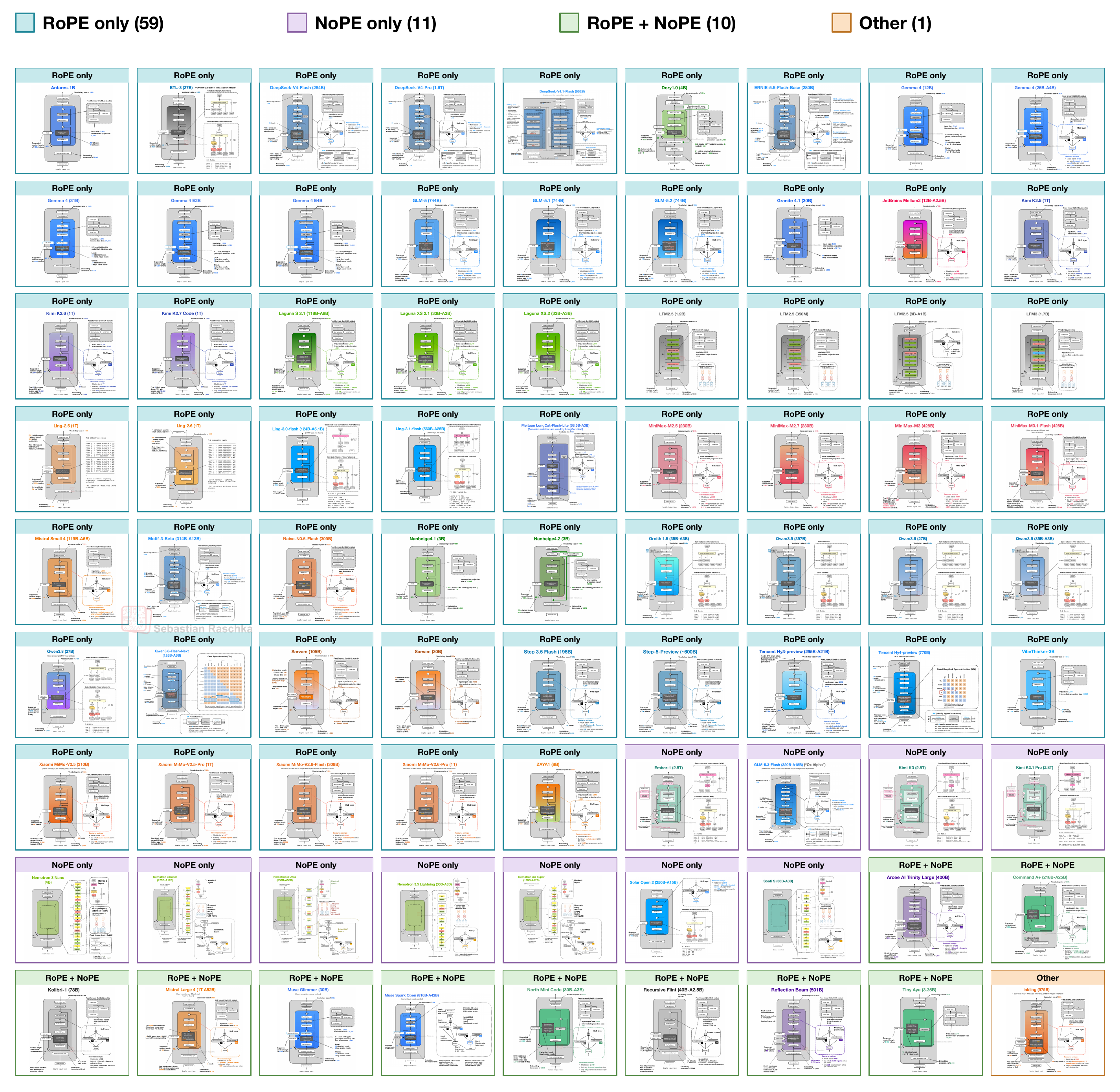
下面你可以看到 2026 年开放权重模型采用了哪些位置嵌入选择的预览。我们会在介绍完底层机制之后再讨论这些选择。
但为什么要花这么多时间来写/读这个相对次要的构建模块呢?LLM 一直在演进,而当我准备今年最新的 LLM 架构趋势新文章时,我意识到自己至今还没有在任何文章中介绍过 LLM 所使用的位置信息方法。所以,与其让另一篇文章变得过于庞杂,我觉得把它作为即将到来的 LLM 架构与趋势分析的独立构建模块单独发表,或许更合理。
另外,多年来许多读者一直希望我写一篇关于相对位置嵌入(即 RoPE)的教程,作为对 GPT 中所用可学习绝对嵌入的后续补充。这件事在我的待办清单上挂了很久,所以我终于重新翻出旧草稿,整理出了这篇讲解,内容将涵盖
LLM 中的不同位置方法;
(终于)RoPE 是如何工作的;
近期开源 LLM 使用了哪些方法。
请注意,本文假定读者对基础 LLM 架构有一定了解,作为《Build a Large Language Model (From Scratch)》的后续阅读材料效果很好。如果你对注意力内部机制的概念与计算,尤其是 query、key、value 向量,还觉得有些模糊,我建议回顾一下我的自注意力讲解作为复习:
这篇文章也相当技术化,对某些人来说可能过于详细。不过,我确实希望把这一基础内容先发布出来,供后续文章引用。别担心,下一篇会回到更轻松易读的风格。
附言:我开始尝试 Substack 新的“perks”系统。作为对支持者的感谢,我添加了架构图库的图片导出和元数据,供你们在自己的分析中使用。
再附言:如果你已经熟悉位置嵌入的工作原理,可以直接跳到第 6 节:现代架构中的位置选择。
请注意,本文在网页浏览器中阅读可能比在邮件客户端中更好。我建议查看这里的网页版,它左侧还有导航栏。
让我们从整体架构开始。分词器(tokenizer)将输入文本编码为 Token ID。接下来,LLM 的输入 Token 嵌入层将这些 ID 分别映射为一个数值向量。我们通常把该向量中的这些元素称为“特征”(类似于经典机器学习)。随后,LLM 内部的 Transformer 块通过注意力和前馈层修改这些向量。最后,模型的输出层为下一个 Token 生成 logit 分数(并转换为概率)。
下图展示了 GPT-2(一个相对经典的 LLM)和 MiniMax-M3(今年发布的较新的 LLM,可代表大多数其他近期 LLM)中的这条路径。可以看到,两者的架构差异并不大,但在进入位置信息部分之前,我们先关注橙色方块(Token 嵌入层)以及其上方的 transformer 块;本次讲解不需要涉及其他架构差异。
如上图所示,Token 嵌入层把每个 Token ID 映射为一个向量,随后再添加位置信息。具体来说(我们稍后会更详细地讨论),GPT-2 会在修改后的嵌入进入第一个 transformer 块之前,为每个 Token 嵌入加上一个位置向量。而 MiniMax-M3 则在每个 transformer 块内部,通过注意力机制中一种名为 RoPE 的方法来添加位置信息。
稍后我们会更详细地讨论这些方法,但首先,让我们从宏观层面说明为什么需要添加显式的位置信息。
以下面两个输入句子作为简单示例:
“The red fox jumps over the gray fox.”
“The gray fox jumps over the red fox.”
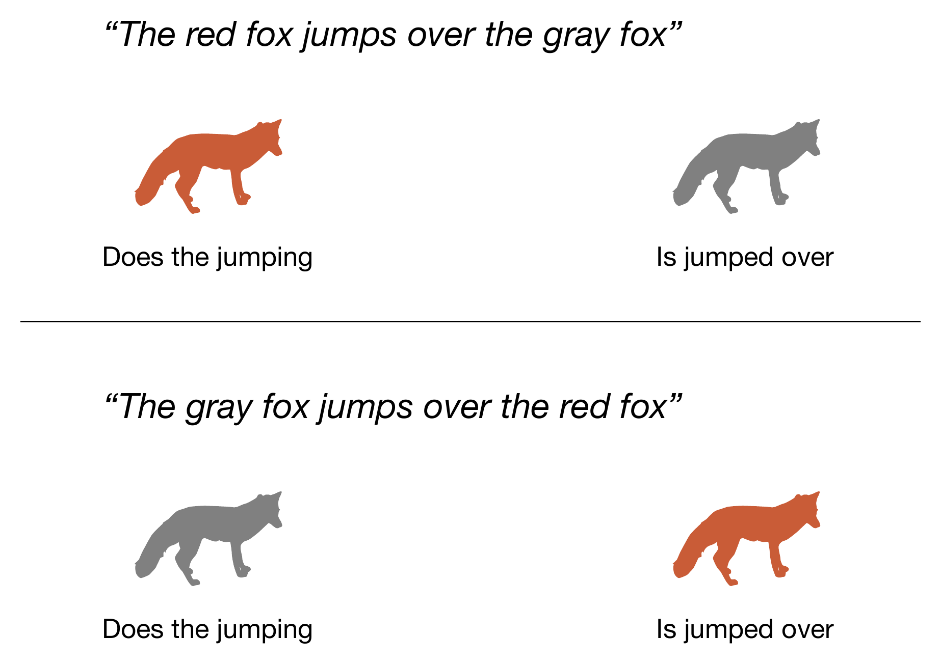
改变词序会改变是哪只狐狸在跳,如下图所示。
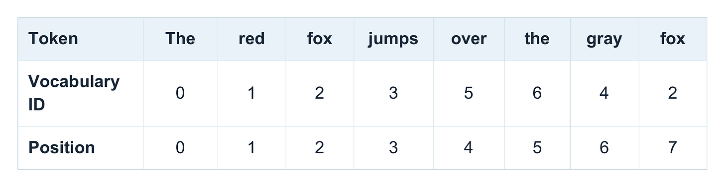
在本文的示例中,为简单起见,我们把每个单词视为一个 Token。(如你所知,真实的分词器可以把单词切分成更小的子词 Token。)这样第一个句子就有八个 Token 位置,从 0 到 7。
# 假设有下面这个小词表。 # 真实的词表通常有 5 万到 20 万条词目 vocab = { "The": 0, "red": 1, "fox": 2, "jumps": 3, "gray": 4, "over": 5, "the": 6, }(如果你对词表是如何构建的感兴趣,可以看看我发在 GitHub 上的分词器资料。)
注意,“fox”在输入句子中出现了两次,两次都得到相同的 Token ID 2。而且由于它们的 Token ID 相同,无论它们在输入句子中处于什么位置,都会从嵌入层得到相同的嵌入向量。
现在,让我们考虑一种不带位置编码(也没有因果掩码)的常规自注意力机制,其中每个输入 Token 都可以关注输入中的所有其他 Token。在这种情况下,交换任意两个词,比如“red”和“gray”,每个 Token 对之间的嵌入和注意力分数仍然相同。
GPT 风格的模型确实使用因果(自回归)掩码,它把每个 Token 限制为只能关注自身和更早的 Token。有趣的是,这种因果掩码给计算带来了一些隐含的顺序信息。在我们的例子里,“jumps”在第一个句子中可以关注“red”,在第二个句子中可以关注“gray”。因此,即使没有显式的位置嵌入,因果 LLM 理论上也已经能够区分这两个句子。(我们稍后讨论“NoPE”概念时会再回到这个想法。)
尽管如此,GPT-2 和大多数较新的 LLM 都包含显式位置信息,因为它为注意力提供了关于位置的直接信号。这是因为,尽管因果掩码决定了哪些 Token 可被访问,并提供了隐式的顺序信息,但它无法区分例如相隔一个位置与相隔十个位置。因此,显式位置方法仍然有用(甚至必不可少),因为它们提供了这类信息。
如果这一切听起来令人困惑,别担心,它更多只是作为概述,我们将在剩余文章中更慢地逐步讲解这些概念。
我们简要讨论了通过因果注意力掩码提供的隐式位置信息(稍后我们会更详细地再次讨论)。然而,现在我们转换话题,讨论添加位置信息的显式方法。
也许最简单、最直接(但并非“最便宜”)的方法是为每个序列位置分配一个自己的向量。我们将该向量加到 Token 嵌入上,因此得到的修改后的嵌入向量随后被传入第一个 Transformer 模块。这一具体过程将在以下小节中讨论。
为了说明如何将显式的、学习得到的位置向量用于输入嵌入,让我们以 GPT-2 作为具体例子。GPT-2 在训练期间学习一个位置向量表。下图展示了这些向量在架构中的使用位置,即在 Token 嵌入查找之后、第一个 Transformer 模块之前。
上图中展示的位置嵌入层与 Token 嵌入层的实现方式相同,即它们具有完全相同的输出维度,因此生成的输入向量可以相互相加。下面的代码展示了这一点,其中包含一段 GPT-2 代码实现:
class GPTModel(nn.Module): def __init__(self, cfg): super().__init__() self.tok_emb = nn.Embedding(cfg["vocab_size"], cfg["emb_dim"]) self.pos_emb = nn.Embedding(cfg["context_length"], cfg["emb_dim"]) self.drop_emb = nn.Dropout(cfg["drop_rate"]) self.trf_blocks = nn.Sequential( *[TransformerBlock(cfg) for _ in range(cfg["n_layers"])]) self.final_norm = LayerNorm(cfg["emb_dim"]) self.out_head = nn.Linear( cfg["emb_dim"], cfg["vocab_size"], bias=False ) def forward(self, in_idx): batch_size, seq_len = in_idx.shape tok_embeds = self.tok_emb(in_idx) pos_embeds = self.pos_emb(torch.arange(seq_len, device=in_idx.device)) x = tok_embeds + pos_embeds # Shape [batch_size, num_tokens, emb_size] x = self.drop_emb(x) x = self.trf_blocks(x) x = self.final_norm(x) logits = self.out_head(x) return logits 用数学术语来说,我们可以将其写为如下形式。设 m 为位置索引,xm 为该位置上的 Token ID。第一个模块的输入是
Etoken 是嵌入层,
Pm 是由 m 选择的位置信息向量,
而 hm 是嵌入向量与位置向量相加后的结果向量。
原文较长,译文为节选;译文由英文原文机器翻译,术语按行业惯例统一,可在文末展开原文核对。
查看英文原文(Understanding Positional Embeddings in Modern LLMs)
This article explains how LLMs encode and process token position information by covering classic and contemporary methods like RoPE. It’s essentially a comprehensive journey where we will work through the mechanisms with visual examples, a little math, and a small PyTorch implementation. And, of course, we will then also look at how modern architectures adapt or omit explicit positional encodings.
Below, you can find a preview of which positional embedding choices are used in 2026 open-weight models. We will discuss these choices later after covering the underlying mechanisms.
But why spending so much time writing/reading about this rather minor building block? LLMs keep evolving, and as I was preparing a new article on the latest LLM architecture trends this year, I realized that I never covered the positional information methods used in LLMs in any article so far. So, instead of letting the other article get out of hand, I thought it might make sense to publish this as a standalone building block for the upcoming LLM architecture and trends analysis.
Also, over the years, many readers have asked me for a tutorial on relative positional embeddings (aka RoPE) to follow up on the learned absolute embeddings used in GPT. It’s been on my TODO list for a long time, so I finally revisited my old draft and put this walkthrough together, which will cover
different positional methods in LLMs;
(finally) how RoPE works;
what methods are used by recent open LLMs.
Note that this article assumes some familiarity with basic LLM architectures and works well as a follow-up to Build a Large Language Model (From Scratch). If the concepts and computation of the attention internals, particularly query, key, and value vectors, are a little fuzzy, I recommend checking my self-attention walkthrough as a refresher:
The article is also very technical and likely too detailed for some. However, I really wanted to have this foundation out there for future articles to reference. And no worries, the next one will return to a more comfortable style.
PS: I started experimenting with Substack’s new “perks” system. As a thank-you to supporters, I’ve added image exports and metadata from the architecture gallery for you to use in your own analyses.
PPS: If you are already familiar with how position embeddings work, feel free to fast-forward to Section 6, Positional choices in modern architectures.
Note that this article may be best read in a web browser than an email client. I recommend checking out the web view here, which also has a navigation bar on the left side.
1. Where position information enters an LLM
Let’s start with the overall architecture. A tokenizer encodes the input text into token IDs. Next, the input token embedding layer of an LLM maps each of these IDs to a vector of numbers. We usually refer to these entries in that vector as “features” (similar to classic ML). The transformer blocks inside the LLM then modify these vectors using attention and feedforward layers. Lastly, the model’s output layer produces logit scores (converted into probabilities) for the next token.
The following shows this path in GPT-2 (a relatively classic LLM) and MiniMax-M3 (a more recent LLM released this year; a placeholder for most other recent LLMs). As we can see, the architectures are not too different from each other, but before we get to the positional information parts, let’s focus on the orange blocks for now (the token embedding layers) and the transformer blocks above them; the other architecture differences aren’t needed for this explanation.
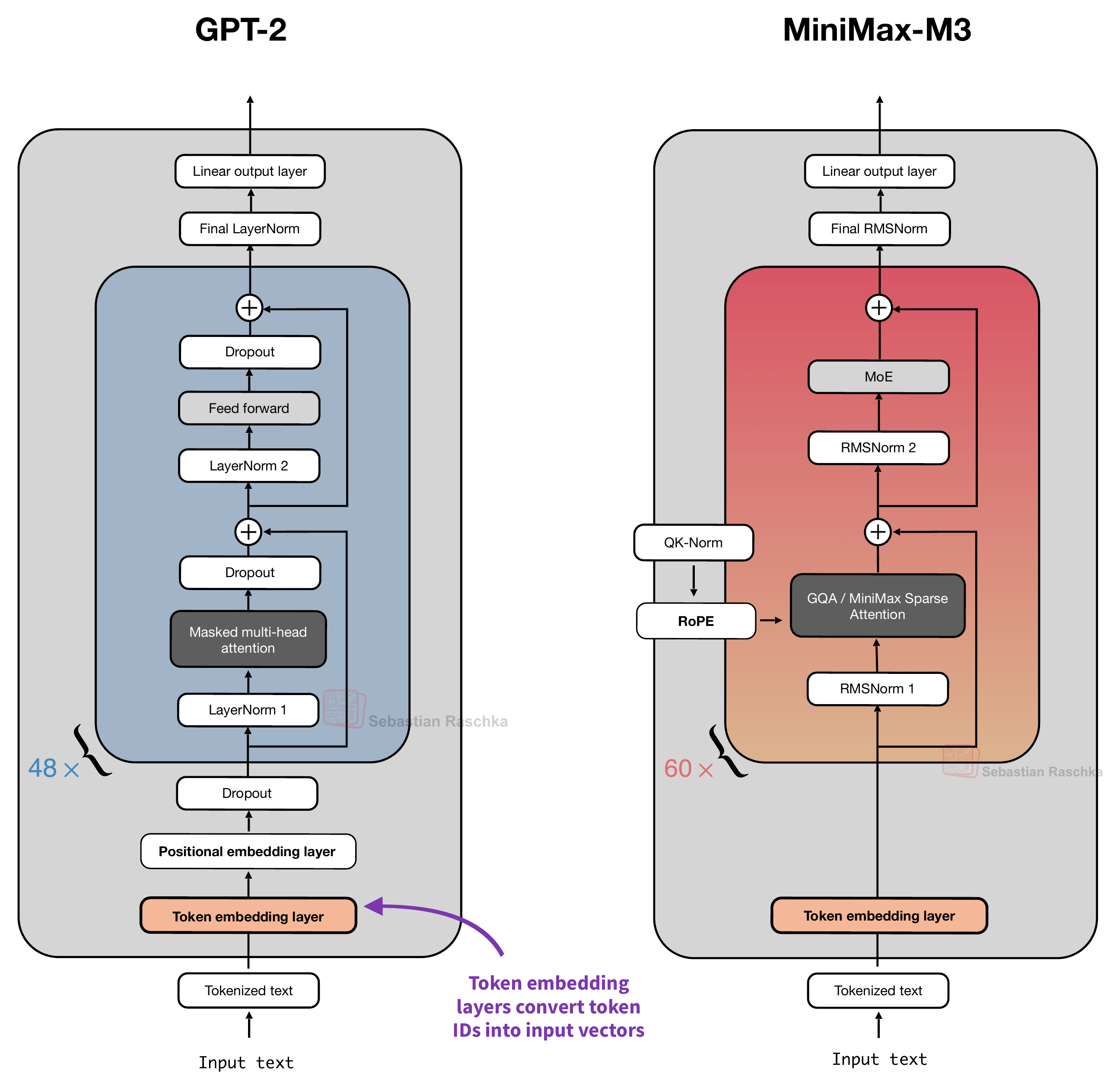
A token embedding layer, shown in the figure above, maps each token ID to a vector. Position information is then added afterward. Concretely, and as we will discuss in more detail later, GPT-2 adds a position vector to each token embedding before the modified embedding enters the first transformer block. On the other hand, MiniMax-M3 adds the positional information in each transformer block using a method called RoPE inside attention.
We will talk about these methods in more detail later, but first, let’s start with the big picture information explaining why explicit positional information is added or needed.
1.1 Why add positional information?
Consider the following two input sentences as a simple example:
“The red fox jumps over the gray fox.”
“The gray fox jumps over the red fox.”
Changing the word order changes which fox does the jumping, as illustrated in the following figure.
For the examples in this article, we will treat each word as one token for simplicity. (As you know, real tokenizers can split words into smaller subword tokens.) The first sentence then has eight token positions, from 0 through 7.
# Assume the following small vocabulary.
# Real vocabularies typically have 50k to 200k entries
vocab = {
    "The": 0,
    "red": 1,
    "fox": 2,
    "jumps": 3,
    "gray": 4,
    "over": 5,
    "the": 6,
}
(If you are interested in how vocabularies are built, check out my tokenizer materials on GitHub.)
Note that “fox”, which appears twice in the input sentence, gets the same token ID 2 in both cases. And since they both have the same token ID, irrespective of the position in the input sentence, they would get the same embedding vector from the embedding layer.
Now, let’s consider a regular self-attention mechanism with no positional encoding (and no causal mask), where every input token can attend to every other token in the input. In this scenario, swapping any two words, like “red” and “gray”, would still result in the same embeddings and attention scores between each token pair.
GPT-style models do use a causal (autoregressive) mask, which restricts each token to itself and earlier tokens. Interestingly, this causal mask gives the computation some implicit order information. In our example, “jumps” can attend to “red” in the first sentence and “gray” in the second. So, a causal LLM can theoretically already distinguish these sentences even without explicit positional embeddings. (We will return to this idea later when discussing the “NoPE” concept.)
Nonetheless, GPT-2 and most newer LLMs include explicit positional information because it gives attention a direct signal about positions. That’s because even though the causal mask determines which tokens are accessible and provides implicit order information, it doesn’t distinguish a separation of one position from a separation of ten, for example. So, explicit positional methods are still useful (or even essential), since they supply that information.
If this all sounded confusing, don’t worry, it was more meant as an overview, and we will step through these concepts a bit more slowly in the remaining article.
2. Adding a position vector to each token embedding
We briefly talked about implicit positional information through causal attention masks (and we will revisit this again in more detail later). However, we now switch gears and talk about the explicit ways to add positional information.
The perhaps simplest and most direct (but not “cheapest”) approach is to give each sequence position its own vector. We add that vector to the token embedding, so the resulting, modified embedding vector is then passed to the first transformer block. This exact procedure is discussed in the following subsections.
2.1 Learned absolute position embeddings in GPT-2
To illustrate the use of an explicit, learned positional vector to the input embeddings, let’s consider GPT-2 as a concrete example. GPT-2 learns a table of position vectors during training. The following figure illustrates where these vectors are used in the architecture, that is, immediately after the token embedding lookup and before the first transformer block.
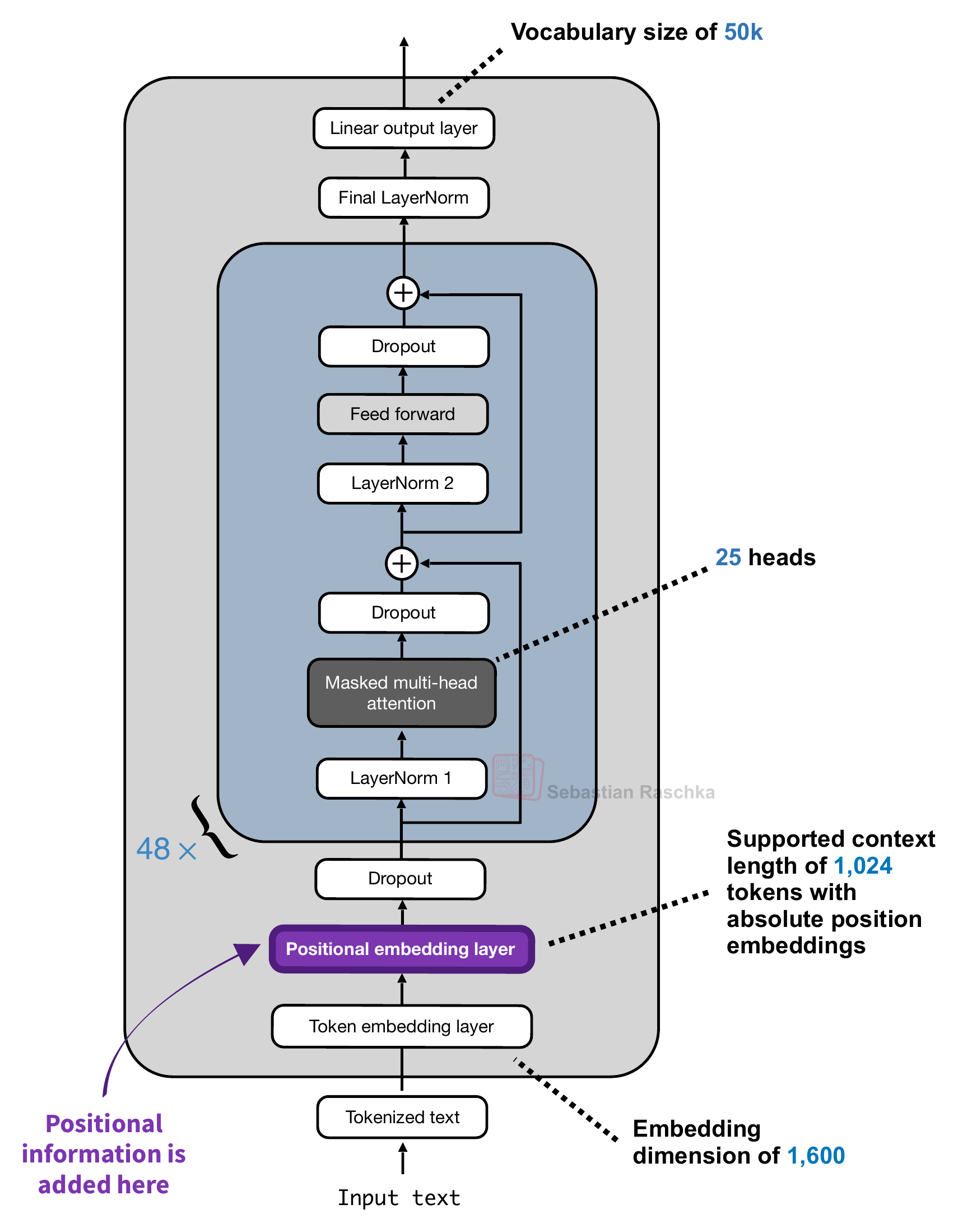
The positional embedding layer depicted in the figure above follows the same implementation as the token embedding layer, i.e., they have exactly the same output dimensions so that the resulting input vectors can be added to each other. The code below shows that with an excerpt of a GPT-2 code implementation:
class GPTModel(nn.Module):
    def __init__(self, cfg):
        super().__init__()
        self.tok_emb = nn.Embedding(cfg["vocab_size"], cfg["emb_dim"])
        self.pos_emb = nn.Embedding(cfg["context_length"], cfg["emb_dim"])
        self.drop_emb = nn.Dropout(cfg["drop_rate"])

        self.trf_blocks = nn.Sequential(
            *[TransformerBlock(cfg) for _ in range(cfg["n_layers"])])

        self.final_norm = LayerNorm(cfg["emb_dim"])
        self.out_head = nn.Linear(
            cfg["emb_dim"], cfg["vocab_size"], bias=False
        )

    def forward(self, in_idx):
        batch_size, seq_len = in_idx.shape
        tok_embeds = self.tok_emb(in_idx)
        pos_embeds = self.pos_emb(torch.arange(seq_len, device=in_idx.device))
        x = tok_embeds + pos_embeds  # Shape [batch_size, num_tokens, emb_size]
        x = self.drop_emb(x)
        x = self.trf_blocks(x)
        x = self.final_norm(x)
        logits = self.out_head(x)
        return logits
And in mathematical terms, we can write it as follows. Let m be a position index and xm the token ID at that position. The input to the first block is

Here,
Etoken is the embedding layer,
Pm is the position info vector selected by m,
and hm is the resulting summed embedding and position vector.
The two vectors have the same width, so we add their entries element-wise. Figure 6 below shows this visually with a small numerical example.
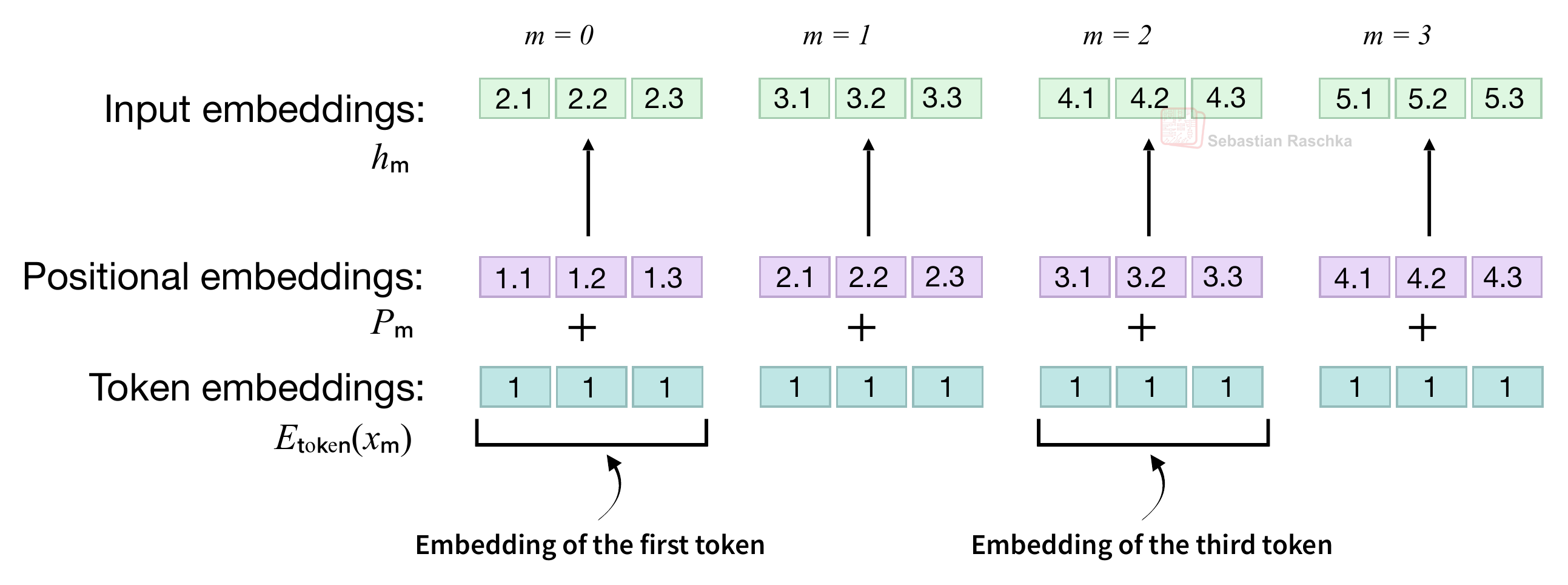
In the figure above, at position 0, adding the token embedding [1, 1, 1] to the position embedding [1.1, 1.2, 1.3] gives [2.1, 2.2, 2.3]. By the way, the values in the figure are chosen to keep the illustration simple; in a real example, both embedding layers (tables) are initialized with small random values and learned during training.
So, what we covered in this section is a so-called absolute positional method because the positional embedding Pm depends on the token’s own position m. In the previous example sentence, the two “fox” tokens have initially the same token embeddings, but because we are adding different positional vectors P2 and P7, they have different values before they enter the first transformer block. And consequently, the query, key, and value vectors inside the attention mechanisms then also receive representations that already include position information.
Note that the original GPT-2 implementation has 1,024 learned position vectors. This means it only works with inputs with 1024 or fewer tokens. If we want to extend the context window, we would have to extend this embedding table. And since the embedding table (layer) is updated like any other layer during training, the context length would have to be decided before the training starts.
Extending the context would be very expensive since the table can become very large. For example, in the case of GPT-2 Medium, the positional embedding layer weights only make up 0.30% of the total weights at 1,024 positions. However, if we increased the context length to a nowadays common 100k range, they would make up >22% of the total model weights, which would be very uneconomic.
2.2 Fixed sinusoidal position encodings in the original transformer
The original “Attention Is All You Need” transformer from 2017, which predates GPT, uses the same addition mechanism, but computes its position vectors with fixed sine and cosine functions. Figure 7 below shows this addition before both the encoder and decoder stacks. The encoder processes the input sequence, and the decoder generates the output sequence. (The reason why it’s introduced here is that the sine and cosine functions will become relevant again later when discussing RoPE.)
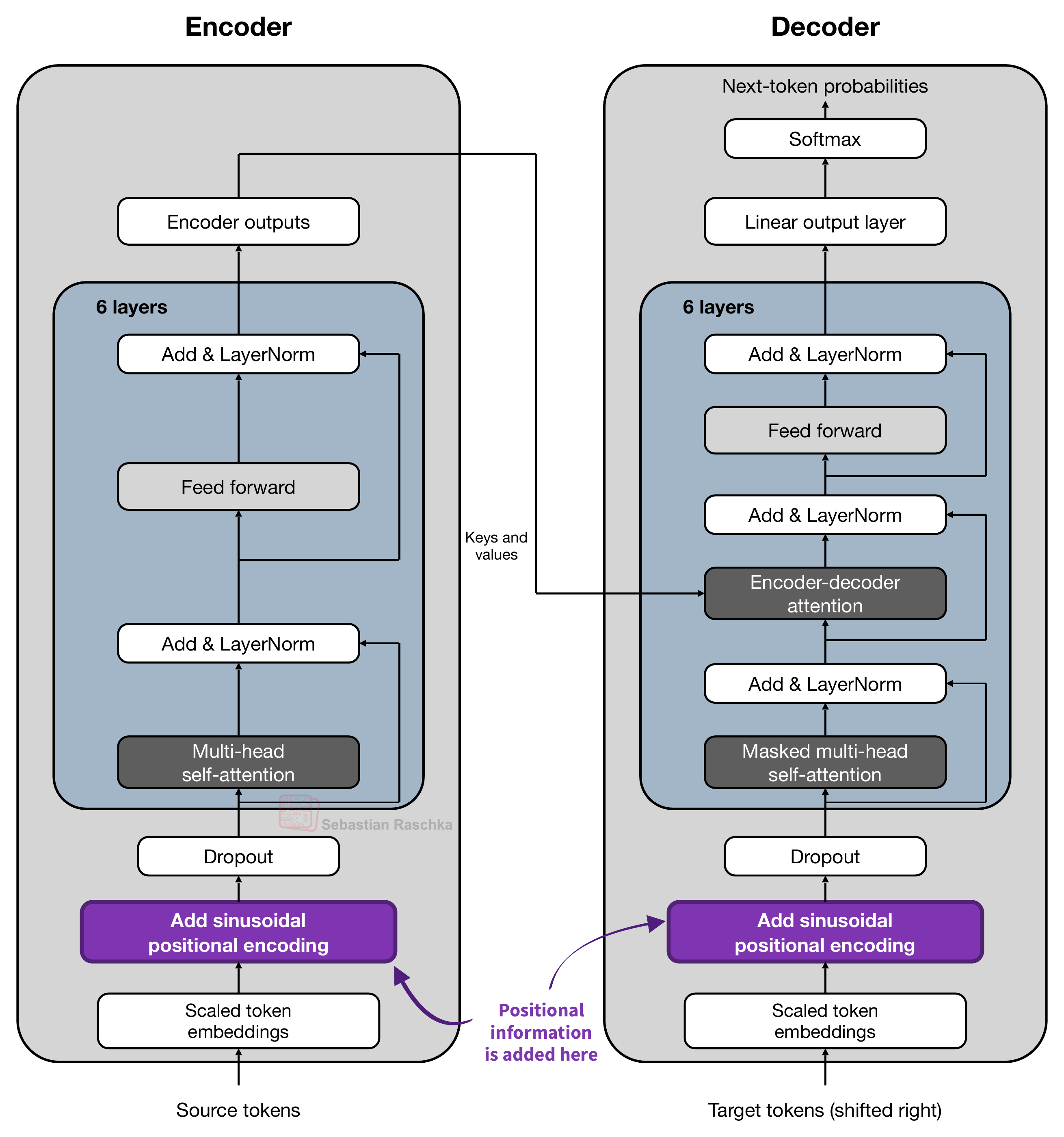
The original transformer also scales its token embeddings by √(dmodel) before adding the position vectors, where dmodel is the embedding width.
So, while GPT-2 in the previous section had the formula
the formula used in the original transformer (depicted in Figure 7) is:

This scaling by √(dmodel) is a minor technical detail, but for those who are curious, the motivation behind this scaling factor is not explained in the transformer paper, but as I discussed with colleagues on a Twitter thread many years ago, it’s likely to put the token embeddings and sinusoidal positional encodings on comparable numerical scales at initialization, so the position vectors don’t dominate the sum when we add them.
In the GPT-2 case, this scaling wasn’t necessary because the original GPT-2 code initialized the token embeddings to have an initial standard deviation of 0.02 and the position embeddings to have an initial standard deviation of 0.01 so that they were already roughly on the same scale.
Now, the more interesting point is how the position embeddings Pm are computed.
Concretely, each position vector has the following entries:

As before, m denotes the position. The index i indexes a pair of features within the vector.
Here, a feature is one number in the position vector. For example, let’s assume we have a small vector with 8 values (dmodel = 8) that has entries numbered 0 through 7. (In the original paper this was 512 for the small model and 1024 for the bigger model, instead of 8, but that would be hard to visualize.) We group these into four pairs so that i goes from 0 through 3.
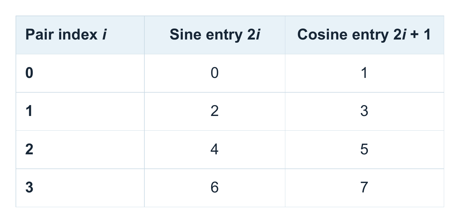
Here, the indices 2i and 2i + 1 select the two entries corresponding to pair i.
As shown in the equation earlier, the angle at position m, which is then fed into the sine or cosine functions to obtain Pm, 2i or Pm, 2i + 1, respectively, is computed as follows:
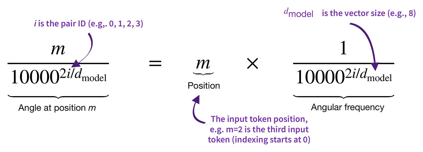
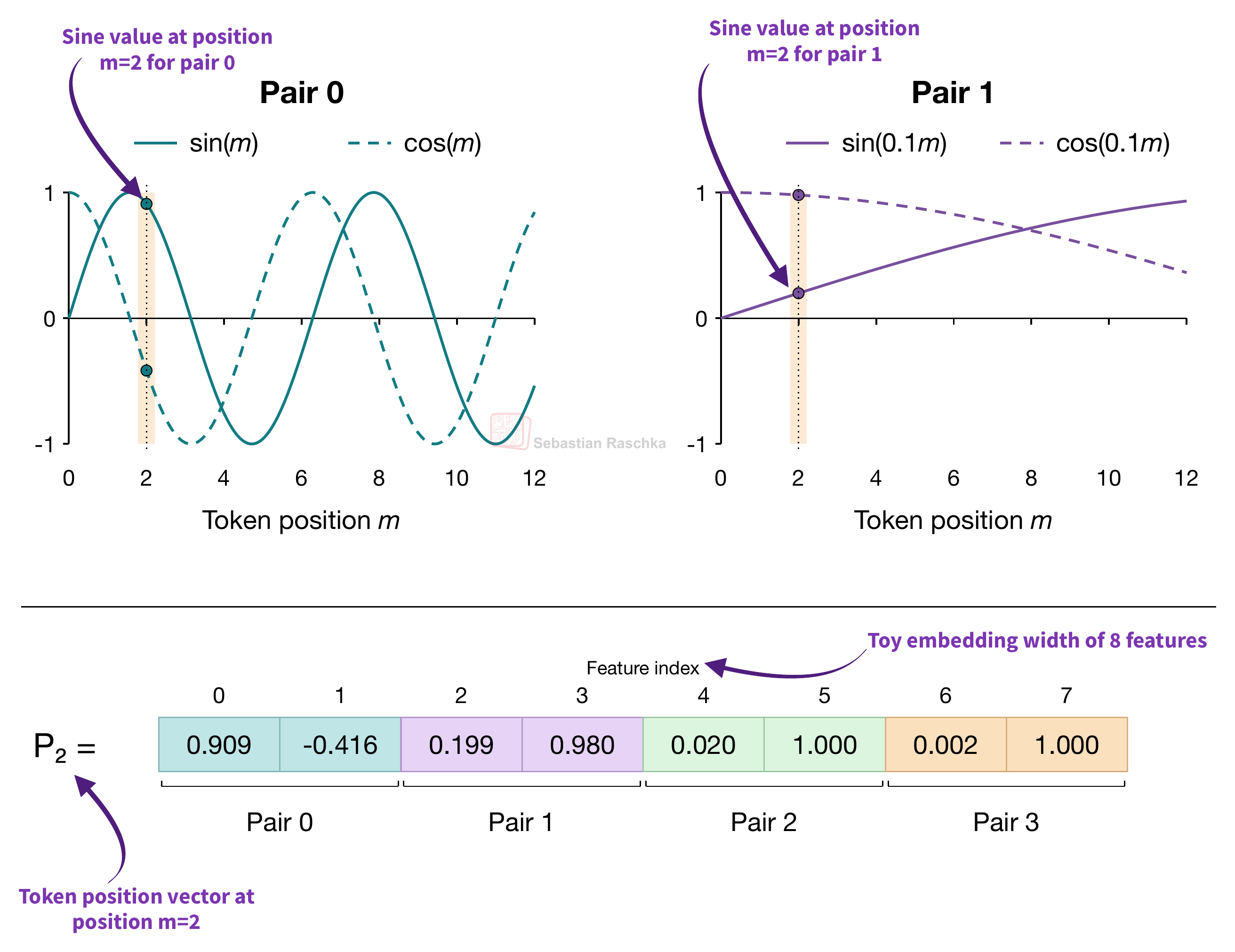
Figure 10 shows this calculation for all four pairs of our 8-feature example at position m = 2.
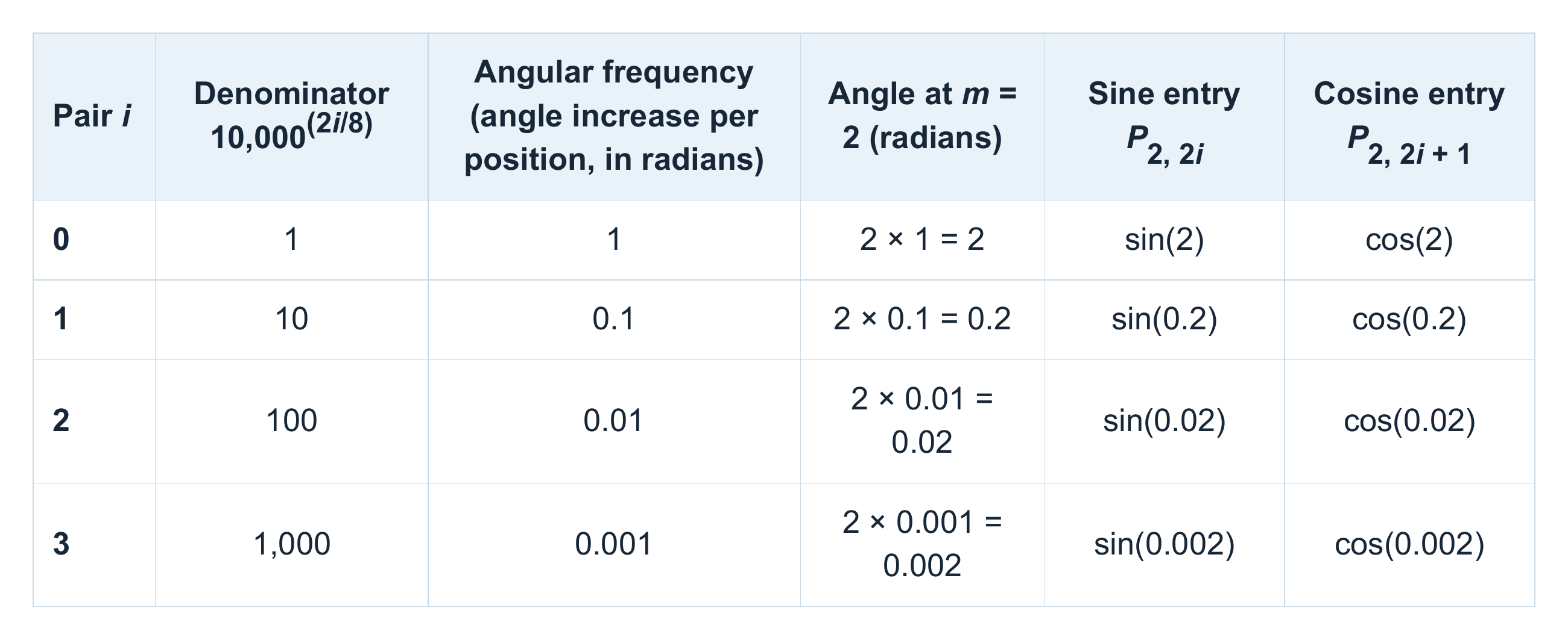
For an eight-feature embedding, the four frequencies are 1, 0.1, 0.01, and 0.001 radians per position. At position 2, the first pair in row 1 is (sin 2, cos 2) ≈ (0.909, −0.416).
The second pair, in row 2, changes more slowly, giving (sin 0.2, cos 0.2) ≈ (0.199, 0.980).
The figure below visualizes the sine and cosine calculations for different pairs, which are then collected in a position vector.
In short, this method is a (more complicated) alternative to obtaining positional embedding vectors compared to the GPT-2 method discussed earlier.
Similar to the GPT-2 embeddings, these are also absolute embeddings because each vector is computed from its own position. However, in contrast to the GPT-2 approach, the sine and cosine functions stay fixed during training. (Also, they can be extended and evaluated beyond the training positions, like beyond the context length of 1024, although that alone doesn’t guarantee that the model will perform well there, because it hasn’t seen those during training.)
To summarize, Figure 12 below compares the two ways of obtaining a position vector we discussed so far.
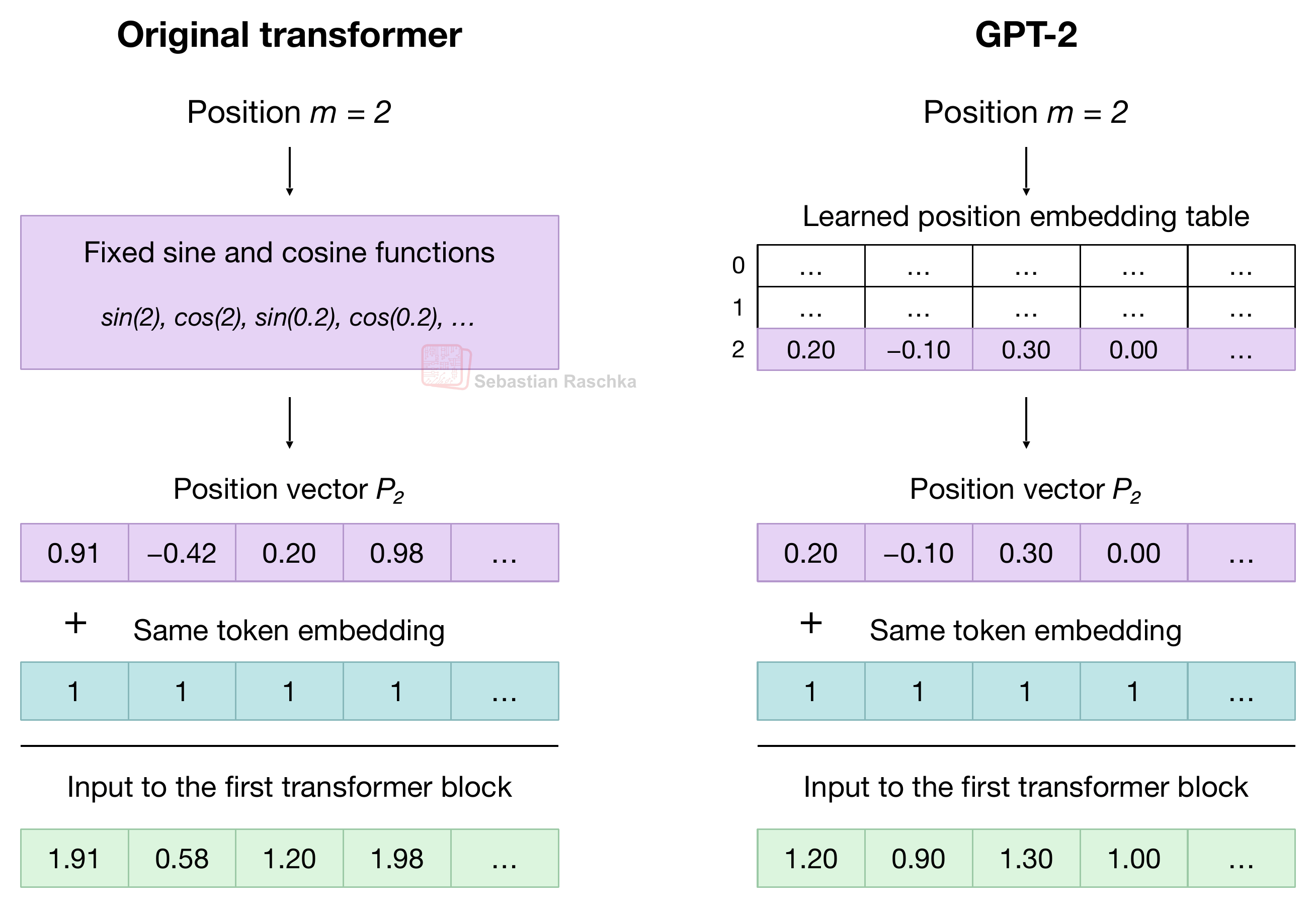
This sinusoidal method may look like an overly complicated way to obtain positional embeddings, however, understanding it will be useful when talking about RoPE in the next section.
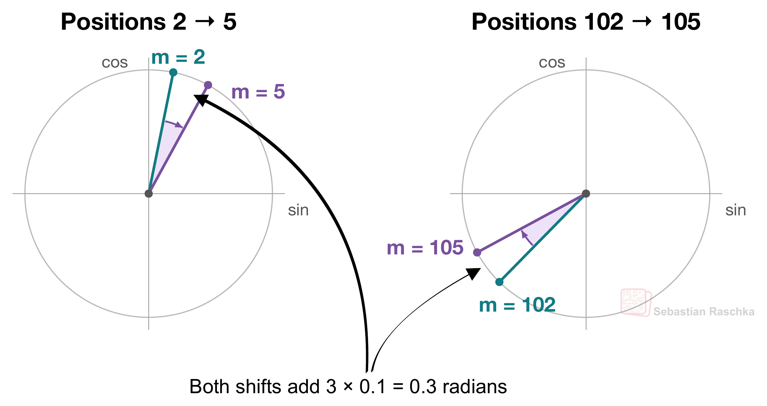
Also, there is some rationale behind it. The authors chose sine and cosine because they make the shifting by a certain offset gives a certain deterministic difference. For example, the difference between position 2 to 5 and the difference between 102 to 105 is both 3, which then results in the same rotation.
According to the Attention Is All You Need paper:
“...easily learn to attend by relative positions, since for any fixed offset k, PEpos + k can be represented as a linear function of PEpos.”
Or in less technical terms, the authors hypothesized that this property would make it easier for attention to learn relationships such as “three tokens earlier.”
Figure 13 below illustrates this for one sine/cosine pair. A rotation is a linear transformation, and both three-position shifts use the same rotation.
3. Encoding relative position with RoPE
So, the sinusoidal method above is still considered an absolute positional encoding because the vector added to each token embedding represents that token’s position counted from the start of the sequence.
As shown in the previous figure, for example, tokens at positions 2 and 5 receive the position vectors P2 and P5. If we move those tokens to positions 102 and 105, they’re still three positions apart. But each token gets a different position vector because its absolute position m has changed.
So their attention score can change even when the token embeddings stay the same. The sinusoidal structure still gives the model a way to learn relative relationships.
Anyways, RoPE, which we will discuss below, builds this relative relationship directly into the attention calculation. RoPE, which Su et al. introduced in the 2021 RoFormer paper, stands for Rotary Position Embedding and is considered a relative position method.
3.1 Moving the rotation inside attention in RoPE
In attention, each token’s current representation is projected into a query, a key, and a value vector. Query-key dot products determine attention scores. After masking and softmax, the resulting weights determine how the value vectors are mixed. For a refresher, see my Understanding and Coding Self-Attention, Multi-Head Attention, Causal-Attention, and Cross-Attention in LLMs article:
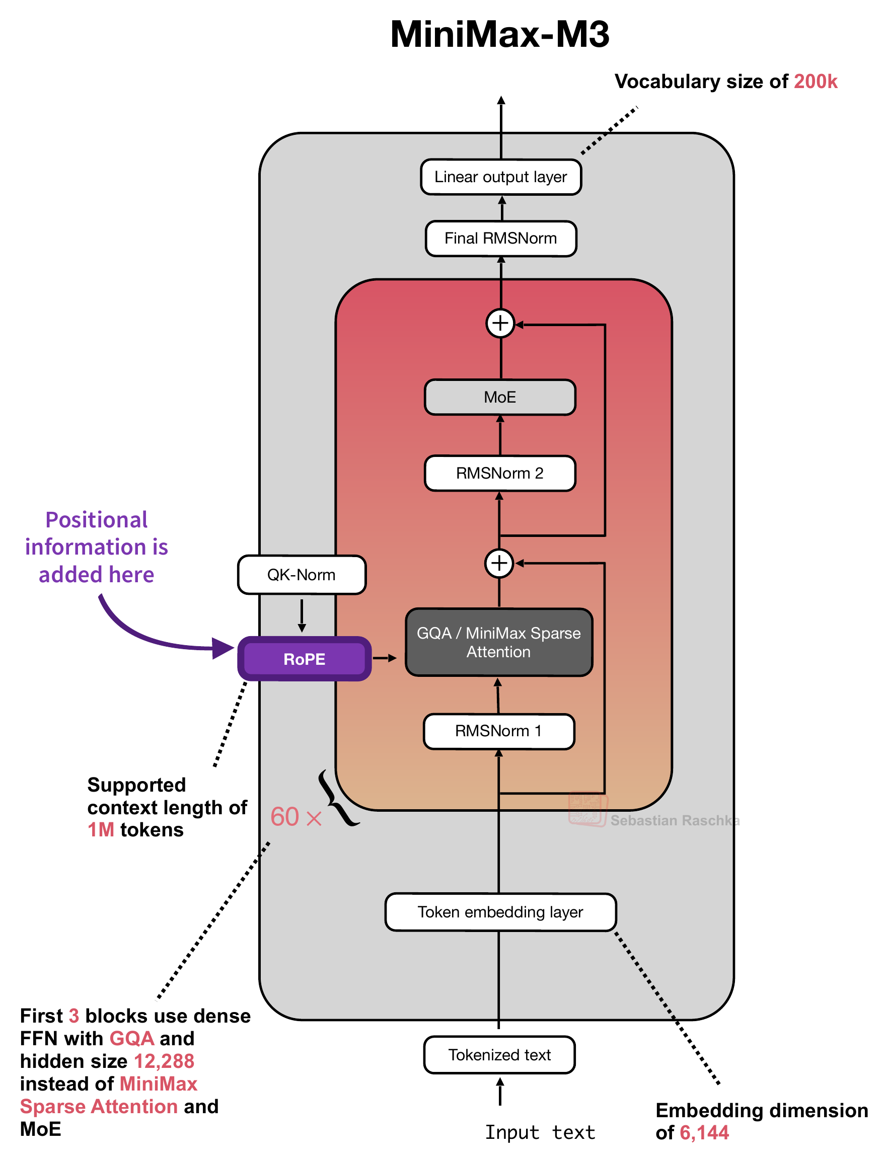
RoPE uses the token’s position to rotate its query and key vectors before their dot product. The value vectors bypass this rotation. Figure 14 below shows an overview of where RoPE is applied in a relatively recent MiniMax-M3, where QK-Norm normalizes queries and keys before RoPE.
 正文保留英文原文,标题与摘要由机器翻译。