OpenFold3 上线 SageMaker JumpStart
你可以通过 Amazon SageMaker JumpStart 部署 OpenFold3-preview。OpenFold Consortium 与哥伦比亚大学 AlQuraishi Lab 共同开发了 OpenFold3,这是一个开源的生物分子结构预测模型。通常只需几行代码,你就能把 OpenFold3 部署到自己的 AWS 账户中。随后你可以预测蛋白质、DNA、RNA、小分子配体及其形成的复合物的三维结构。该端点以网络隔离方式运行,你可以借此帮助把序列保留在自己的 AWS 账户内。
如今,计算药物发现团队把结构预测作为其工作的核心部分。团队将其用于靶点识别、抗体与蛋白质工程以及基于结构的虚拟筛选。团队发现运行这些模型颇具挑战:你需要 GPU 基础设施、可正常工作的 CUDA 与 PyTorch 软件栈、大型模型检查点,以及一个能处理耗时以分钟而非毫秒计的请求的服务层。SageMaker JumpStart 可以为你承担其中大量工作。OpenFold3 在 AWS 维护的容器中运行,部署在托管的 Amazon SageMaker AI 端点上。该端点旨在处理请求排队与 GPU 预热,你还可以添加自动扩缩容。
在这篇文章中,我们将向你展示如何:
OpenFold3 是一个全原子结构预测模型。它根据一组分子的序列预测它们共同的 3D 结构。它并不局限于单条蛋白质链:它能在一次预测中折叠多链蛋白质复合物、蛋白质–核酸组装体以及蛋白质–配体复合物。
OpenFold3 的开发者以 Apache 2.0 许可证发布其代码和模型权重,并公开训练数据与方法。研究机构和制药公司可以依照该许可证的条款检查该模型、对其进行微调,并在其基础上继续开发。开发者将 OpenFold3-preview 描述为一个研究预览版。
大多数 JumpStart 模型,例如大语言模型和嵌入模型,都部署到实时端点。实时端点在一次请求内返回响应,且该请求被限制在 60 秒以内。结构预测的工作方式则不同。折叠时间会随查询中链的数量和长度而增加,而真实世界的蛋白质和复合物往往需要数分钟。
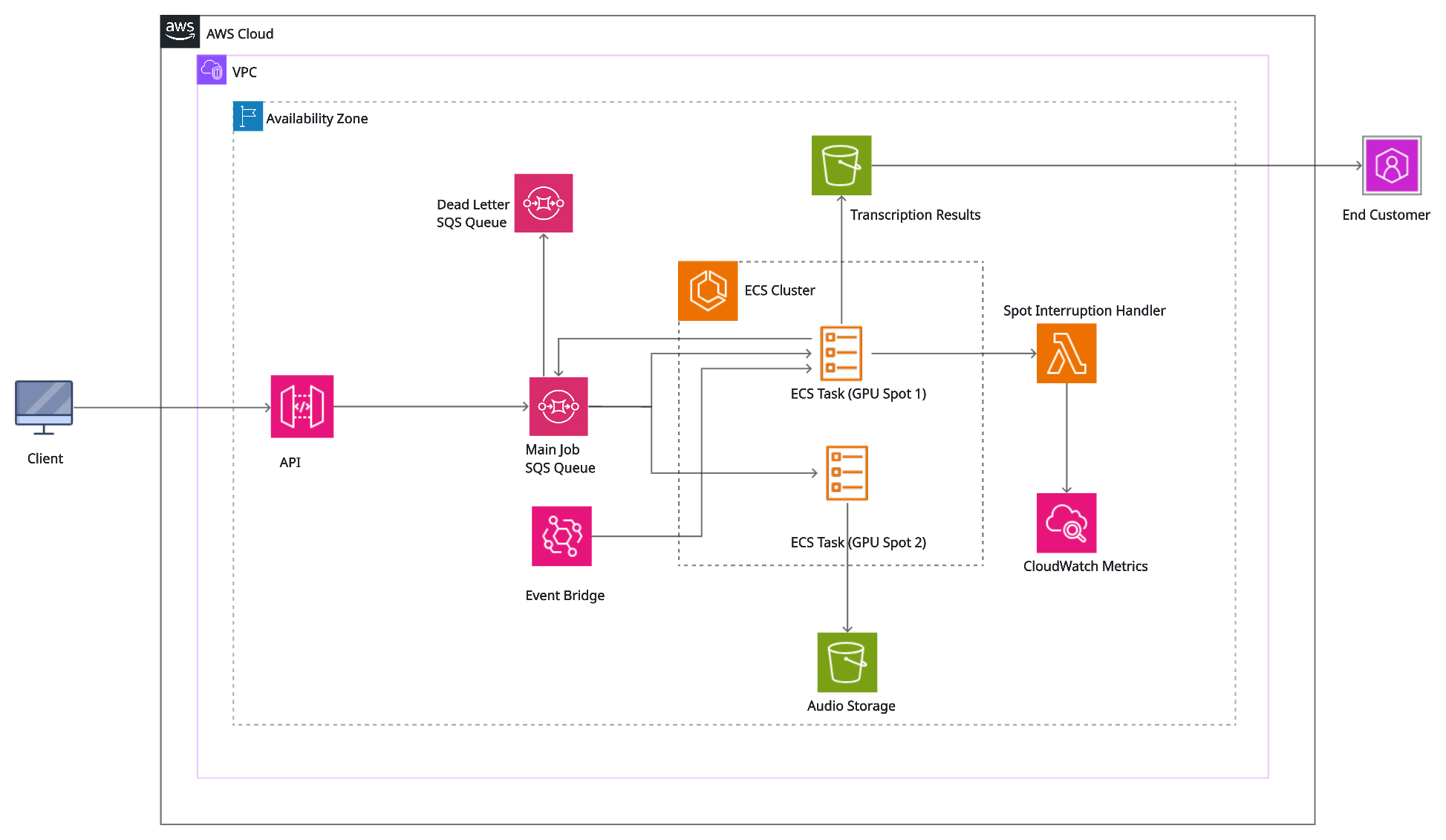
因此,JumpStart 上的 OpenFold3 运行在 SageMaker Asynchronous Inference 上:
异步端点的两个特性特别适合科学计算负载。第一,它们在内部对突发请求进行排队,因此你可以提交一大批序列,而无需自建作业队列。第二,当队列为空时,它们可以缩容至零实例,这有助于避免为实验间隙的空闲实例付费。
要跟随本演练操作,你需要:
重要提示:SageMaker 端点在运行期间按实例小时计费,包括空闲期间。为避免意外费用,请遵循“清理”部分,或按本文后文所述配置缩容至零。有关定价详情,请参阅 Amazon SageMaker AI 定价。
首先,依据其 JumpStart 配置构建模型,并定义一个 AsyncInferenceConfig。输出路径和失败路径是端点写入结果和错误详情的 S3 位置。
import json, time, uuid import boto3 from sagemaker.core.helper.session_helper import Session from sagemaker.core.inference_config import AsyncInferenceConfig from sagemaker.core.jumpstart.configs import JumpStartConfig from sagemaker.core.training.configs import Compute from sagemaker.serve.model_builder import ModelBuilder session = Session() bucket = session.default_bucket() # sagemaker-{region}-{account-id} prefix = "openfold3-async" model_builder = ModelBuilder.from_jumpstart_config( jumpstart_config=JumpStartConfig( model_id="huggingface-proteinfolding-openfold3", accept_eula=True, ), compute=Compute(instance_type="ml.g6.4xlarge"), ) model = model_builder.build() async_config = AsyncInferenceConfig( output_path=f"s3://{bucket}/{prefix}/output", failure_path=f"s3://{bucket}/{prefix}/failure", ) endpoint = model_builder.deploy(inference_config=async_config) endpoint_name = endpoint.endpoint_name print(f"Deployed asynchronous endpoint: {endpoint_name}") 设置 accept_eula=True 表示你已查看并接受该模型的许可条款,这是部署此模型所必需的。如果你在 SageMaker Studio 之外运行这段代码,还需通过 role_arn="<role-arn>" 将你的 SageMaker 执行角色传给 ModelBuilder.from_jumpstart_config。
该端点会将你的请求和结果存储在 Amazon S3 中,其中包含你的序列和预测结构。对于专有序列,建议使用专用的 S3 存储桶或前缀,并使用由你管理的 AWS Key Management Service(AWS KMS)密钥进行服务端加密。若要使用你自己的密钥加密结果,请将其 ARN 作为 kms_key_id 传给 AsyncInferenceConfig。通过存储桶策略限制访问,仅允许运行此工作流的角色访问,并添加 S3 生命周期规则,使不再需要保留的请求和结果对象过期。更多信息,请参阅 Amazon S3 安全最佳实践。
部署通常会在几分钟内完成。这包括一个预热步骤,容器会在每个 GPU 上运行一次简短预测,这样当端点进入 InService 状态时,GPU 已经预热完毕。
提示:G6 容量在某些区域可能受限。如果部署因 InsufficientInstanceCapacity 而失败,可稍后重试、选择其他受支持的实例规格,或在该模型可用的其他 AWS 区域部署。
一个请求是一份 JSON 文档,其中包含一个或多个具名查询,每个查询列出其链。一个查询中的所有链会一并折叠为一个复合物。不同查询则各自独立折叠。
每条链包含以下字段:
以下示例折叠人类泛素(ubiquitin),这是一种特征明确的 76 个残基的蛋白质:
s3 = boto3.client("s3") smr = boto3.client("sagemaker-runtime") payload = { "queries": { "ubiquitin": { "chains": [ { "molecule_type": "protein", "chain_ids": ["A"], "sequence": "MQIFVKTLTGKTITLEVEPSDTIENVKAKIQDKEGIPPDQQRLIFAGKQLEDGRTLSDYNIQKESTLHLVLRLRGG", } ] } } } # 1. Stage the request in S3 input_key = f"{prefix}/input/{uuid.uuid4().hex}.json" s3.put_object(Bucket=bucket, Key=input_key, Body=json.dumps(payload).encode()) # 2. Submit asynchronously -- returns immediately resp = smr.invoke_endpoint_async( EndpointName=endpoint_name, ContentType="application/json", InputLocation=f"s3://{bucket}/{input_key}", InvocationTimeoutSeconds=3600, ) output_location, failure_location = resp["OutputLocation"], resp["FailureLocation"] 然后轮询 S3 以获取结果或失败记录:
def split(uri): b, _, k = uri.removeprefix("s3://").partition("/") return b, k result = None for _ in range(120): # up to ~30 minutes for loc, is_failure in ((output_location, False), (failure_location, True)): try: body = s3.get_object(Bucket=split(loc)[0], Key=split(loc)[1])["Body"].read() except s3.exceptions.NoSuchKey: continue if is_failure: raise RuntimeError(body.decode()) result = json.loads(body) if result: break time.sleep(15) if result is None: raise TimeoutError(f"No result yet; check {output_location}") if result.get("status") == "error": raise RuntimeError(result["error"]) 带有无效输入的请求,例如格式错误的链或不受支持的 MSA 名称,仍会产生一个结果对象,但其中会包含 "status": "error" 和一条错误消息,而不是结构。最后一次检查会显现该消息。
预测时间随输入规模增长而增加。在我们对 ml.g6.4xlarge 的测试中,较小的蛋白质比较大型蛋白质完成得更快。
响应包含一个状态、一个 mmCIF 格式的预测结构列表,以及它们对应的置信度。默认情况下,OpenFold3 会为每次查询生成五个扩散样本,因此每次查询返回五个候选结构。每个样本都附带两个置信度文件:一个详细文件(*_confidences.json)和一个摘要文件(*_confidences_aggregated.json)。摘要中包含 sample_ranking_score,你可以用它来选择最佳样本。
import os os.makedirs("structures", exist_ok=True) for s in result["structures"]: path = os.path.join("structures", os.path.basename(s["filename"])) with open(path, "w") as f: f.write(s["content"]) print("saved", path, f'({s["size_bytes"]/1024:.0f} KB)') summaries = {c["filename"]: c["data"] for c in result["confidences"] if c["filename"].endswith("_aggregated.json")} for name, m in sorted(summaries.items(), key=lambda kv: -kv[1]["sample_ranking_score"]): print(f'{name}: ranking={m["sample_ranking_score"]:.2f} pLDDT={m["avg_plddt"]:.1f} ' f'pTM={m["ptm"]:.2f} ipTM={m["iptm"]:.2f}') 你可以在任何结构查看器中打开 .cif 文件,例如 PyMOL、ChimeraX 或 Mol*。要在笔记本中内联查看结构,请使用 py3Dmol:
原文较长,译文为节选;译文由英文原文机器翻译,术语按行业惯例统一,可在文末展开原文核对。
查看英文原文(OpenFold3 on Amazon SageMaker JumpStart: Predict biomolecular structures)
You can deploy OpenFold3-preview from Amazon SageMaker JumpStart. The OpenFold Consortium and the AlQuraishi Lab at Columbia University developed OpenFold3 as an open source biomolecular structure prediction model. With a few lines of code, you can typically deploy OpenFold3 into your own AWS account. You can then predict the 3D structures of proteins, DNA, RNA, small-molecule ligands, and the complexes they form. The endpoint runs with network isolation, which you can use to help keep your sequences within your AWS account.
Computational drug discovery teams now use structure prediction as a core part of their work. Teams use it in target identification, antibody and protein engineering, and structure-based virtual screening. Teams have found running these models challenging. You need GPU infrastructure, a working CUDA and PyTorch stack, large model checkpoints, and a serving layer that handles requests that take minutes rather than milliseconds. SageMaker JumpStart can handle much of that work for you. OpenFold3 runs in an AWS-maintained container on a managed Amazon SageMaker AI endpoint. The endpoint is designed to handle request queuing and GPU warmup, and you can add autoscaling.
In this post, we show you how to:
- Deploy OpenFold3-preview on a SageMaker asynchronous inference endpoint.
- Submit structure prediction jobs and interpret the results, including predicted structures and confidence scores.
- Run several predictions in parallel on multi-GPU instances.
- Supply your own multiple sequence alignments (MSAs) to improve prediction accuracy while helping keep your sequences private.
- Help reduce costs by scaling your endpoint to zero when it’s idle.
Overview of OpenFold3
OpenFold3 is an all-atom structure prediction model. It predicts the joint 3D structure of a set of molecules from their sequences. It isn’t limited to single protein chains: It can fold multi-chain protein complexes, protein–nucleic acid assemblies, and protein–ligand complexes in one prediction.
| Attribute | Details |
| Developer | OpenFold Consortium / AlQuraishi Lab, Columbia University |
| Model type | All-atom biomolecular structure prediction |
| Inputs | Protein, DNA, and RNA sequences. Small-molecule ligands as SMILES |
| Outputs | Predicted structures in mmCIF format, with confidence metrics (pLDDT, PAE, PDE) |
| Version | OpenFold3 0.4.1, of3-p2-155k checkpoint |
| License | Apache 2.0 |
| JumpStart model ID | huggingface-proteinfolding-openfold3 |
| Supported instances | ml.g6.2xlarge, ml.g6.4xlarge (default), ml.g6.12xlarge |
The OpenFold3 developers release its code and model weights under the Apache 2.0 license, and they publish the training data and methods. Research organizations and pharmaceutical companies can inspect the model, fine-tune it, and build on it under the terms of that license. The developers describe OpenFold3-preview as a research preview.
Use cases
- Target and complex structure prediction – Predict structures for targets that have no experimental structure, including multi-chain assemblies and protein–nucleic acid complexes.
- Protein–ligand co-folding – Fold a protein together with a small molecule supplied as SMILES to generate binding-pose hypotheses for structure-based design.
- Antibody and protein engineering – Evaluate designed variants by predicting their structures and comparing confidence across candidates.
- High-throughput screening pipelines – Queue large batches of prediction jobs against an autoscaling endpoint and process the results directly from Amazon Simple Storage Service (Amazon S3).
Why OpenFold3 uses asynchronous inference
Most JumpStart models, such as large language models and embedding models, deploy to real-time endpoints. A real-time endpoint returns its response within a single request, and that request is capped at 60 seconds. Structure prediction works differently. Folding time grows with the number and length of the chains in a query, and real-world proteins and complexes often take several minutes.
For this reason, OpenFold3 on JumpStart runs on SageMaker Asynchronous Inference:
- You upload the request to Amazon S3 and call
InvokeEndpointAsync, which returns immediately. - The endpoint queues the request and processes it, with an invocation timeout of up to 1 hour.
- The endpoint writes the result, or the error details, to an S3 location you choose. You can poll for it or get a notification through Amazon Simple Notification Service (Amazon SNS).
Two properties of asynchronous endpoints suit scientific workloads especially well. First, they queue bursts of requests internally, so you can submit a large batch of sequences without building your own job queue. Second, they can scale to zero instances when the queue is empty, which helps you avoid paying for idle instances between experiments.
Prerequisites
To follow this walkthrough, you need:
- An AWS account, and a SageMaker AI execution role for the endpoint. Following least privilege, this AWS Identity and Access Management (IAM) role needs read and write access only to the S3 prefix that you use for requests and results. For more information, see How to use SageMaker AI execution roles.
- IAM permissions for the identity that runs the code: to create, describe, invoke, and delete the model, endpoint configuration, and endpoint, plus
iam:PassRolefor the execution role. For the optional scale-to-zero section, it also needs AWS Application Auto Scaling and Amazon CloudWatch alarm permissions. In production, scope these permissions to your resources rather than using broad managed policies such asAmazonSageMakerFullAccess. For more information, see Complete the prerequisites for asynchronous inference. - Access to Amazon SageMaker Studio, a SageMaker notebook instance, or a local IDE.
- The SageMaker Python SDK v3 and py3Dmol, which you can install with
pip install "sagemaker>=3,<4" py3Dmol. - Service quota for at least one
ml.g6.4xlargeendpoint instance in your AWS Region. You also need quota forml.g6.12xlargeif you follow the multi-GPU section. You can check your quotas and request increases in the Service Quotas console under Amazon SageMaker.
Important: SageMaker endpoints are billed per instance-hour while they’re running, including while they’re idle. To avoid unexpected charges, follow the Clean up section, or configure scale-to-zero as described later in this post. For pricing details, see Amazon SageMaker AI pricing.
Discover OpenFold3 in SageMaker JumpStart
- Open SageMaker Studio and choose JumpStart in the navigation pane.
- Search for OpenFold3.
- Open the model card to review the model description, license, and supported instance types.
- Open the example notebook from the model card. It contains the complete asynchronous deployment walkthrough shown in this post.
Deploy OpenFold3 with the SageMaker Python SDK
First, build the model from its JumpStart configuration and define an AsyncInferenceConfig. The output and failure paths are the S3 locations where the endpoint writes results and error details.
import json, time, uuid
import boto3
from sagemaker.core.helper.session_helper import Session
from sagemaker.core.inference_config import AsyncInferenceConfig
from sagemaker.core.jumpstart.configs import JumpStartConfig
from sagemaker.core.training.configs import Compute
from sagemaker.serve.model_builder import ModelBuilder
session = Session()
bucket = session.default_bucket() # sagemaker-{region}-{account-id}
prefix = "openfold3-async"
model_builder = ModelBuilder.from_jumpstart_config(
jumpstart_config=JumpStartConfig(
model_id="huggingface-proteinfolding-openfold3",
accept_eula=True,
),
compute=Compute(instance_type="ml.g6.4xlarge"),
)
model = model_builder.build()
async_config = AsyncInferenceConfig(
output_path=f"s3://{bucket}/{prefix}/output",
failure_path=f"s3://{bucket}/{prefix}/failure",
)
endpoint = model_builder.deploy(inference_config=async_config)
endpoint_name = endpoint.endpoint_name
print(f"Deployed asynchronous endpoint: {endpoint_name}")Setting accept_eula=True confirms that you’ve reviewed and accepted the model’s license terms, which is required to deploy this model. If you run this code outside SageMaker Studio, also pass your SageMaker execution role to ModelBuilder.from_jumpstart_config with role_arn="<role-arn>".
The endpoint stores your requests and results in Amazon S3, and they contain your sequences and predicted structures. For proprietary sequences, consider using a dedicated S3 bucket or prefix with server-side encryption using an AWS Key Management Service (AWS KMS) key that you manage. To encrypt results with your key, pass its ARN to AsyncInferenceConfig as kms_key_id. Restrict access with a bucket policy that allows only the roles that run this workflow, and add an S3 Lifecycle rule to expire request and result objects that you don’t need to keep. For more information, see Security best practices for Amazon S3.
Deployment typically completes within minutes. This includes a warmup step in which the container runs a short prediction on each GPU, so that the GPUs are warmed up when the endpoint reaches InService.
Tip: G6 capacity can be limited in some Regions. If a deployment fails with
InsufficientInstanceCapacity, retry later, choose a different supported instance size, or deploy in another AWS Region where the model is available.
Run a structure prediction
A request is a JSON document with one or more named queries, and each query lists its chains. All chains in a query are folded together as one complex. Separate queries are folded independently.
Each chain has these fields:
molecule_type–protein,dna,rna, orligand.chain_ids– a list of chain identifiers, such as["A"]. To specify identical copies, such as a homodimer, use["A", "B"].sequence– the residue sequence, for protein, DNA, and RNA chains.smiles– a SMILES string, used for ligand chains instead ofsequence.
The following example folds human ubiquitin, a well-characterized 76-residue protein:
s3 = boto3.client("s3")
smr = boto3.client("sagemaker-runtime")
payload = {
"queries": {
"ubiquitin": {
"chains": [
{
"molecule_type": "protein",
"chain_ids": ["A"],
"sequence": "MQIFVKTLTGKTITLEVEPSDTIENVKAKIQDKEGIPPDQQRLIFAGKQLEDGRTLSDYNIQKESTLHLVLRLRGG",
}
]
}
}
}
# 1. Stage the request in S3
input_key = f"{prefix}/input/{uuid.uuid4().hex}.json"
s3.put_object(Bucket=bucket, Key=input_key, Body=json.dumps(payload).encode())
# 2. Submit asynchronously -- returns immediately
resp = smr.invoke_endpoint_async(
EndpointName=endpoint_name,
ContentType="application/json",
InputLocation=f"s3://{bucket}/{input_key}",
InvocationTimeoutSeconds=3600,
)
output_location, failure_location = resp["OutputLocation"], resp["FailureLocation"]Then poll S3 for either the result or a failure record:
def split(uri):
b, _, k = uri.removeprefix("s3://").partition("/")
return b, k
result = None
for _ in range(120): # up to ~30 minutes
for loc, is_failure in ((output_location, False), (failure_location, True)):
try:
body = s3.get_object(Bucket=split(loc)[0], Key=split(loc)[1])["Body"].read()
except s3.exceptions.NoSuchKey:
continue
if is_failure:
raise RuntimeError(body.decode())
result = json.loads(body)
if result:
break
time.sleep(15)
if result is None:
raise TimeoutError(f"No result yet; check {output_location}")
if result.get("status") == "error":
raise RuntimeError(result["error"])A request with invalid input, such as a malformed chain or an unsupported MSA name, still produces a result object, but with "status": "error" and an error message instead of structures. The last check surfaces that message.
Prediction time grows with the size of the input. In our tests on ml.g6.4xlarge, smaller proteins completed more quickly than larger proteins.
Interpret the results
The response contains a status, a list of predicted structures in mmCIF format, and their matching confidences. By default, OpenFold3 generates five diffusion samples per query, so each query returns five candidate structures. Each sample comes with two confidence files: a detailed one (*_confidences.json) and a summary (*_confidences_aggregated.json). The summary includes a sample_ranking_score that you can use to pick the best sample.
import os
os.makedirs("structures", exist_ok=True)
for s in result["structures"]:
path = os.path.join("structures", os.path.basename(s["filename"]))
with open(path, "w") as f:
f.write(s["content"])
print("saved", path, f'({s["size_bytes"]/1024:.0f} KB)')
summaries = {c["filename"]: c["data"] for c in result["confidences"]
if c["filename"].endswith("_aggregated.json")}
for name, m in sorted(summaries.items(), key=lambda kv: -kv[1]["sample_ranking_score"]):
print(f'{name}: ranking={m["sample_ranking_score"]:.2f} pLDDT={m["avg_plddt"]:.1f} '
f'pTM={m["ptm"]:.2f} ipTM={m["iptm"]:.2f}')You can open the .cif files in any structure viewer, such as PyMOL, ChimeraX, or Mol*. To view a structure inline in a notebook, use py3Dmol:
import py3Dmol   # pip install py3Dmol
view = py3Dmol.view(width=600, height=450)
view.addModel(result["structures"][0]["content"], "cif")
# pLDDT is stored in the B-factor field: red = low confidence, blue = high
view.setStyle({"cartoon": {"colorscheme": {"prop": "b", "gradient": "roygb", "min": 50, "max": 90}}})
view.zoomTo(); view.show()
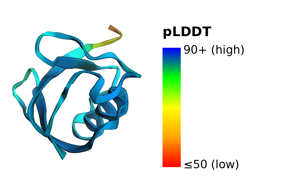
Figure 1: OpenFold3’s predicted structure of ubiquitin, rendered with the preceding code and colored by per-atom confidence (pLDDT). All figures in this post were rendered with 3Dmol.js (Rego and Koes, Bioinformatics, 2015).
The prediction shows ubiquitin’s compact fold: a mixed beta-sheet packed against a single alpha-helix. Most of the structure is blue (high confidence). Only the flexible C-terminal tail, at the top of the image, shifts toward yellow and red, which matches the tail’s known flexibility in experimental structures.
The confidence metrics tell you how much to trust each prediction:
- pLDDT (predicted local distance difference test) – Per-atom confidence in the local structure, on a scale of 0–100. Higher is better, and values above about 70 generally indicate a reliable local structure. The summary file reports the average as
avg_plddt. - pTM and ipTM (predicted TM-score and interface pTM) – Overall confidence in the fold, and in how chains and ligands are positioned relative to each other, on a scale of 0–1. For complexes, ipTM is the key number. The summary file also reports
chain_pair_iptmfor each pair of chains. - PAE (predicted aligned error) and PDE (predicted distance error) – Per-residue-pair error estimates, in the detailed confidence file. Use them to judge the relative placement of domains and chains.
Fold a complex
To predict a complex, list several chains in the same query. The following example co-folds human carbonic anhydrase II with its catalytic zinc ion and the drug acetazolamide. This is a well-studied complex with experimental structures in the Protein Data Bank (for example, PDB 3HS4):
ca2_sequence = (
    "MSHHWGYGKHNGPEHWHKDFPIAKGERQSPVDIDTHTAKYDPSLKPLSVSYDQATSLRILNNGHAFNVEFDDSQDKAVLKGG"
    "PLDGTYRLIQFHFHWGSLDGQGSEHTVDKKKYAAELHLVHWNTKYGDFGKAVQQPDGLAVLGIFLKVGSAKPGLQKVVDVLDS"
    "IKTKGKSADFTNFDPRGLLPESLDYWTYPGSLTTPPLLECVTWIVLKEPISVSSEQVLKFRKLNFNGEGEPEELMVDNWRPAQ"
    "PLKNRQIKASFK"
)

payload = {
    "queries": {
        "ca2_acetazolamide": {
            "chains": [
                {"molecule_type": "protein", "chain_ids": ["A"], "sequence": ca2_sequence},
                {"molecule_type": "ligand",  "chain_ids": ["B"], "smiles": "[Zn+2]"},
                {"molecule_type": "ligand",  "chain_ids": ["C"], "smiles": "CC(=O)Nc1nnc(s1)S(=O)(=O)N"},
            ]
        }
    }
}
Protein sequences in these examples are from UniProt (P0CG48, P00918). You submit and read this request the same way as the ubiquitin example. For complexes like this one, prediction quality depends heavily on providing an MSA, as the next sections show.
Run predictions in parallel on multi-GPU instances
A single OpenFold3 prediction runs on one GPU, so a multi-GPU instance doesn’t make an individual prediction faster. Instead, you can run several predictions at once. On a multi-GPU instance such as ml.g6.12xlarge, which has four GPUs, the container assigns each concurrent request its own GPU. To use all the GPUs, set max_concurrent_invocations_per_instance to the number of GPUs on the instance (four, for ml.g6.12xlarge):
multi_gpu_builder = ModelBuilder.from_jumpstart_config(
    jumpstart_config=JumpStartConfig(
        model_id="huggingface-proteinfolding-openfold3",
        accept_eula=True,
    ),
    compute=Compute(instance_type="ml.g6.12xlarge"),
)
multi_gpu_model = multi_gpu_builder.build()

async_config = AsyncInferenceConfig(
    output_path=f"s3://{bucket}/{prefix}/output",
    failure_path=f"s3://{bucket}/{prefix}/failure",
    max_concurrent_invocations_per_instance=4,   # = number of GPUs on the instance
)

multi_gpu_endpoint = multi_gpu_builder.deploy(inference_config=async_config)
This creates a second endpoint, so remember to delete it as well when you’re done (see Clean up).
In our tests, four concurrent predictions each ran on a separate GPU, with throughput gains that grew with protein size. For larger proteins, the cost per prediction that we measured on ml.g6.12xlarge, based on On-Demand instance pricing, was close to that of ml.g6.4xlarge. Your results depend on your inputs and Region. For pricing, see Amazon SageMaker AI pricing.
Note:
ml.g6.12xlargecapacity can be limited. If it isn’t available in your Region, you can increase throughput by scaling out across severalml.g6.4xlargeinstances with the autoscaling configuration described later in this post.
Use the following table to choose an instance:
| Workload | Recommended instance | Why |
| Interactive exploration by a single user | ml.g6.2xlarge or ml.g6.4xlarge |
One GPU handles one prediction at a time at the lowest hourly cost of the supported instances |
| Team use or bursts of concurrent requests | ml.g6.12xlarge with max_concurrent_invocations_per_instance=4 |
Four predictions run in parallel instead of queuing |
| High-throughput screening | ml.g6.12xlarge with autoscaling |
Highest throughput per instance of the supported instances. Scales out with queue depth and back to zero |
Improve prediction accuracy with your own MSAs
OpenFold3 can take a multiple sequence alignment (MSA) as an additional input for each protein chain. An MSA is a set of evolutionarily related sequences aligned to your query. Co-variation across those sequences signals which residues are likely to be in contact, so MSAs can substantially improve accuracy for many proteins and complexes.
To help keep your sequences within your AWS account, the JumpStart endpoint runs with network isolation and doesn’t call external MSA servers. Instead, it accepts precomputed MSAs in the request. You generate alignments with the pipeline and sequence databases you already use, on infrastructure you control, and pass them to the endpoint. This design can help drug discovery programs that need to keep proprietary sequences private.
If you don’t supply an MSA, the endpoint predicts from the sequence alone. That can work well for small, well-characterized proteins such as ubiquitin. For most real-world targets and complexes, include an MSA. The rest of this section shows how, and how much it improves results.
Bring your own MSA
Each protein chain accepts a precomputed_msa field: a list of alignments, each with a name and the alignment content in A3M or Stockholm format. For a single merged alignment, such as the output of a ColabFold MMseqs2 search, use the name colabfold_main:
with open("ca2_colabfold.a3m") as f:
    ca2_msa = f.read()

payload["queries"]["ca2_acetazolamide"]["chains"][0]["precomputed_msa"] = [
    {"name": "colabfold_main", "content": ca2_msa}
]
This example has one protein chain. If a query has several different protein chains, compute an MSA for each one and attach it to that chain’s precomputed_msa field. Identical copies listed together under one chain_ids entry, such as a homodimer, share a single MSA.
The endpoint also accepts other alignment names, such as uniref90_hits, mgnify_hits, and bfd_uniclust_hits, if you generate MSAs with a different pipeline. Because the request is staged in S3, you can send large alignments. In our tests, alignments of several megabytes worked.
You can generate MSAs with tools such as ColabFold (MMseqs2) or HHblits or JackHMMER. To help keep proprietary sequences inside your environment, run the search on your own AWS infrastructure against locally hosted sequence databases, rather than sending sequences to a public server. For example, ColabFold’s colabfold_batch command uses the public ColabFold MSA server by default, so for proprietary sequences, use colabfold_search with locally hosted databases instead.
How much difference does an MSA make?
We folded the carbonic anhydrase II, zinc, and acetazolamide complex from the previous section twice on the same endpoint: once in single-sequence mode, and once with an MSA from a ColabFold MMseqs2 search.
| Metric (first of 5 samples) | Without MSA | With MSA |
| Average pLDDT | 30 | 98 |
| pTM | 0.22 | 0.98 |
| ipTM | 0.49 | 0.98 |
| Zinc–His94/His96/His119 distance | 2.3–9.4 Å | 2.0 Å each |
| Acetazolamide nitrogen–zinc distance | 5.6 Å | 2.0 Å |
| Prediction time | ~1.5 minutes | ~1.5 minutes |
With the MSA, OpenFold3 recovers the known binding mode. The zinc ion is coordinated by the three active-site histidines, and the acetazolamide sulfonamide nitrogen binds directly to the zinc, matching the experimental structure. Without the MSA, the protein fold has low confidence and the binding site isn’t formed. Adding the MSA didn’t noticeably change prediction time.
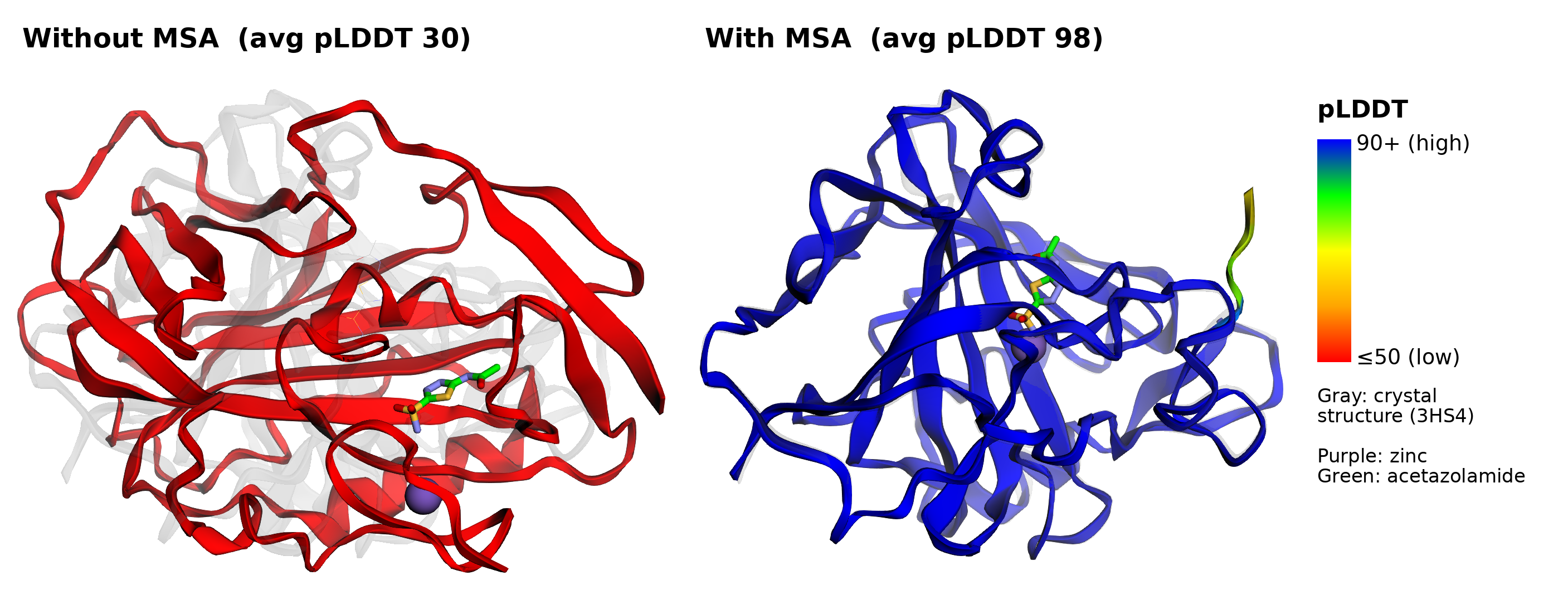
Figure 2: The same carbonic anhydrase II, zinc, and acetazolamide query folded without an MSA (left) and with an MSA (right). Each prediction is colored by pLDDT and superimposed on the experimental crystal structure (gray, PDB 3HS4; Sippel et al., 2009).
Superimposed on the crystal structure, the MSA-based prediction matches it closely: the protein backbone deviates by 0.2 Å (Cα RMSD), the zinc ion by less than 0.1 Å, and the acetazolamide heavy atoms by 0.4 Å RMSD. The single-sequence prediction is misfolded, with a Cα RMSD of 22 Å.
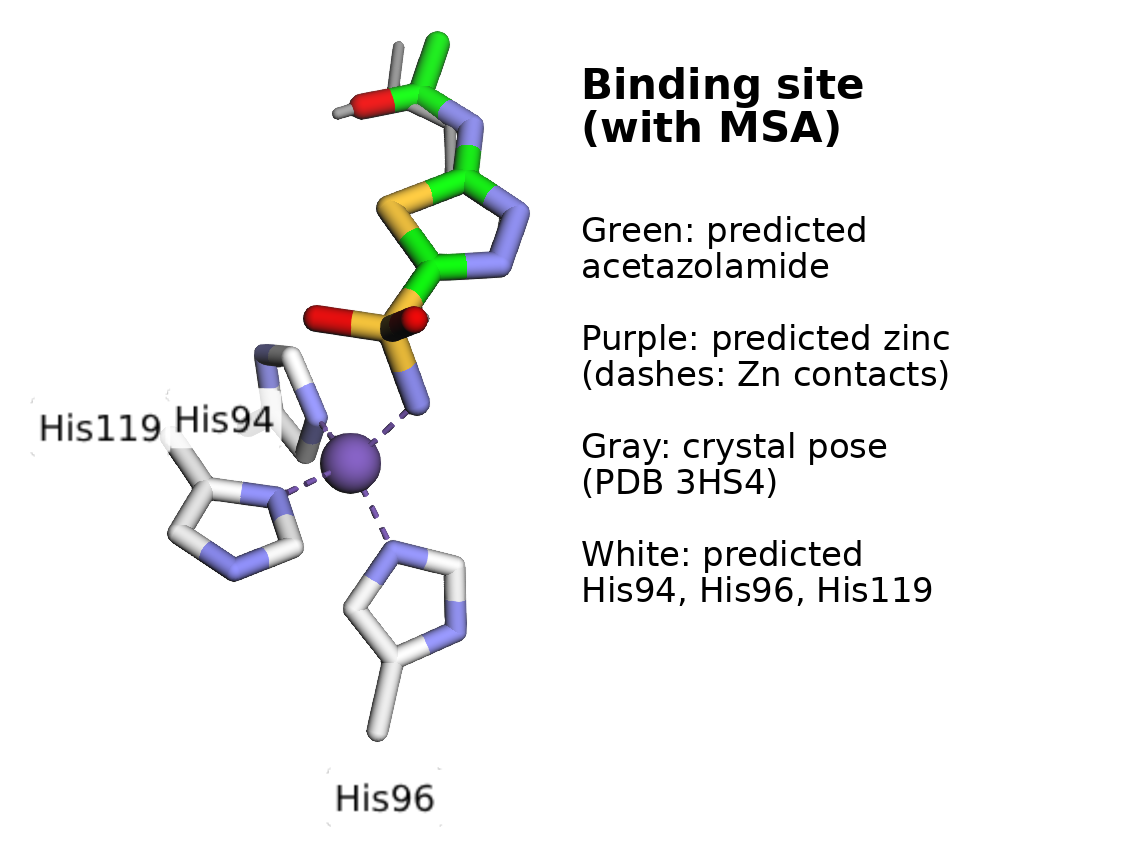
Figure 3: Close-up of the binding site in the MSA-based prediction. The predicted zinc ion (purple) is coordinated by His94, His96, and His119 and by the sulfonamide nitrogen of acetazolamide (green). The crystal pose (gray) is almost entirely hidden behind the prediction.
Carbonic anhydrase II with acetazolamide is one of the most extensively studied complexes in the Protein Data Bank, and closely related structures are likely part of OpenFold3’s training data. Treat this example as a demonstration of the workflow and of how much an MSA matters, not as a benchmark of accuracy on novel targets.
When you compare OpenFold3 results against other tools or published benchmarks, compare like with like: single-sequence results with single-sequence results, and MSA-based results with MSA-based results.
Help reduce cost: Scale to zero when idle
Asynchronous endpoints can scale down to zero instances when no requests are queued, and scale back up when new requests arrive. This pattern suits structure prediction work, which often runs in bursts.
aas = boto3.client("application-autoscaling")
resource_id = f"endpoint/{endpoint_name}/variant/AllTraffic"

aas.register_scalable_target(
    ServiceNamespace="sagemaker",
    ResourceId=resource_id,
    ScalableDimension="sagemaker:variant:DesiredInstanceCount",
    MinCapacity=0,
    MaxCapacity=4,
)

# Scale out and in to keep about 4 queued requests per instance
aas.put_scaling_policy(
    PolicyName="openfold3-backlog",
    ServiceNamespace="sagemaker",
    ResourceId=resource_id,
    ScalableDimension="sagemaker:variant:DesiredInstanceCount",
    PolicyType="TargetTrackingScaling",
    TargetTrackingScalingPolicyConfiguration={
        "TargetValue": 4.0,
        "CustomizedMetricSpecification": {
            "MetricName": "ApproximateBacklogSizePerInstance",
            "Namespace": "AWS/SageMaker",
            "Dimensions": [{"Name": "EndpointName", "Value": endpoint_name}],
            "Statistic": "Average",
        },
        "ScaleInCooldown": 600,
        "ScaleOutCooldown": 300,
    },
)
Target tracking scales the endpoint down to zero after the queue has been empty for a while. In our tests, that took about 15–20 minutes. However, target tracking doesn’t scale the endpoint back up from zero. To start an instance when a request arrives and no instances are running, add a step-scaling policy that’s triggered by the HasBacklogWithoutCapacity metric:
cw = boto3.client("cloudwatch")

step = aas.put_scaling_policy(
    PolicyName="openfold3-scale-from-zero",
    ServiceNamespace="sagemaker",
    ResourceId=resource_id,
    ScalableDimension="sagemaker:variant:DesiredInstanceCount",
    PolicyType="StepScaling",
    StepScalingPolicyConfiguration={
        "AdjustmentType": "ChangeInCapacity",
        "MetricAggregationType": "Average",
        "Cooldown": 300,
        "StepAdjustments": [{"MetricIntervalLowerBound": 0, "ScalingAdjustment": 1}],
    },
)

cw.put_metric_alarm(
    AlarmName=f"{endpoint_name}-has-backlog-without-capacity",
    Namespace="AWS/SageMaker",
    MetricName="HasBacklogWithoutCapacity",
    Dimensions=[{"Name": "EndpointName", "Value": endpoint_name}],
    Statistic="Average",
    Period=60,
    EvaluationPeriods=2,
    DatapointsToAlarm=2,
    Threshold=1,
    ComparisonOperator="GreaterThanOrEqualToThreshold",
    TreatMissingData="missing",
    AlarmActions=[step["PolicyARN"]],
)
When a request arrives at an endpoint with zero instances, it waits in the queue while an instance starts. The first request after scaling from zero will take longer to complete as it includes time for the alarm to trigger, the instance to start, plus the prediction itself. Later requests in the same burst run at normal speed. This trade-off can work well for batch workloads. For interactive use, set MinCapacity=1 to keep one instance warm. For more details, see Autoscale an asynchronous endpoint.
Clean up
To stop incurring charges, delete the resources you created when you’re finished. If you configured autoscaling, remove it first: delete the Amazon CloudWatch alarm, then deregister the scalable target. Then delete each endpoint, its endpoint configuration, and its model, including the multi-GPU endpoint if you deployed it:
# 1. If you configured autoscaling, remove it before deleting the endpoint
cw.delete_alarms(AlarmNames=[f"{endpoint_name}-has-backlog-without-capacity"])
aas.deregister_scalable_target(
    ServiceNamespace="sagemaker",
    ResourceId=resource_id,
    ScalableDimension="sagemaker:variant:DesiredInstanceCount",
)

# 2. Delete the endpoints, endpoint configurations, and models
#    (include only the ones you deployed)
from sagemaker.core.resources import EndpointConfig

for m, ep in ((model, endpoint), (multi_gpu_model, multi_gpu_endpoint)):
    endpoint_config = EndpointConfig.get(endpoint_config_name=ep.endpoint_name)
    m.delete()
    ep.delete()
    endpoint_config.delete()
If you no longer need the request and result objects, you can also delete them from s3://<bucket>/openfold3-async/.
Conclusion
With OpenFold3 on SageMaker JumpStart, research and drug discovery teams can deploy an open, inspectable structure prediction model into their own AWS account with a few lines of code. Asynchronous inference handles long-running folds and bursty batch workloads, and multi-GPU instances run predictions in parallel. Network isolation helps you keep proprietary sequences private, and because you can bring your own MSAs, you can benefit from MSAs without sending sequences to an external server. With scale-to-zero, you stop paying for endpoint instances after the queue has been empty long enough for the endpoint to scale in. Other charges, such as for Amazon S3 storage, still apply.
The code in this post is sample code for experimentation. Before you use it with proprietary or regulated data, work with your security and legal teams to meet your organization’s security, regulatory, and compliance requirements.
To get started, search for OpenFold3 in SageMaker JumpStart, or open the example notebook from the model card. To learn more about the features used in this post, see Asynchronous inference and Autoscale an asynchronous endpoint. To discuss your structural biology workloads, contact your AWS account team.
About the authors

Malav Shastri
Malav Shastri is a Software Development Engineer at AWS, where he builds the infrastructure that brings open source and proprietary foundation models (text, vision, audio, and video) to customers through Amazon SageMaker JumpStart. Over the past 5+ years, he has worked across the ML stack, from SageMaker workflows and containers to model deployment, fine-tuning pipelines, and multi-agent systems that automate model onboarding. He is most interested in model serving and the infrastructure that makes ML reliable and fast in production.

Manu Pillai
Manu is a Sr. Specialist Solutions Architect at AWS, focused on high-performance computing and cloud solutions for life sciences organizations. With over 12 years of experience in the life sciences industry, he brings deep domain expertise to help organizations leverage cloud technologies to advance scientific discovery.

Kevin Wang
Kevin is a Software Development Engineer on the AWS Deep Learning Containers/AMIs team, where he builds and maintains deep learning images that customers run on Amazon Elastic Compute Cloud (Amazon EC2), Amazon SageMaker AI, and Amazon Elastic Kubernetes Service (Amazon EKS). His team manages the images and their build systems as open source on GitHub.

Anamaria Todor
Anamaria is a Principal Solutions Architect based in Copenhagen, Denmark. She saw her first computer when she was 4 years old and never let go of computer science, video games, and engineering since. She has worked in various technical roles, from freelancer, full-stack developer, to data engineer, technical lead, and CTO, at various companies in Denmark, focusing on the gaming and advertising industries. She has been at AWS for over 5 years, working as a Principal Solutions Architect, focusing mainly on life sciences and AI/ML. Anamaria has a bachelor’s in Applied Engineering and Computer Science, a master’s degree in Computer Science, and over 10 years of AWS experience. When she’s not working or playing video games, she’s coaching girls and female professionals in understanding and finding their path through technology.
Zhuofu Bai
Zhuofu is a Software Development Manager at AWS.
正文保留英文原文,标题与摘要由机器翻译。
原文发布于 AWS Machine Learning(OpenFold3 on Amazon SageMaker JumpStart: Predict biomolecular structures),标题、摘要与正文由机器翻译,术语按行业惯例统一,未经人工逐句校订。