文本分类语言模型:从词袋到 Jev
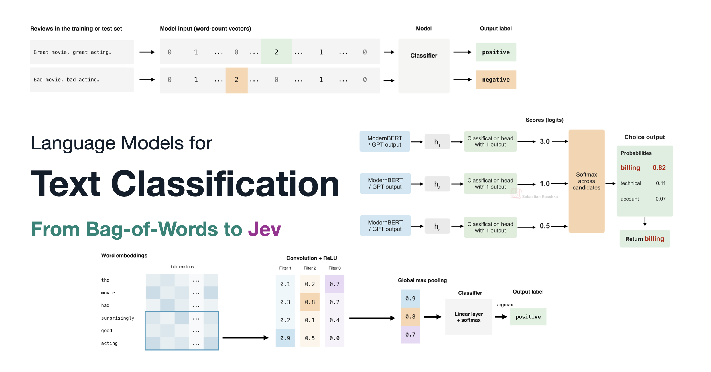
最近发布的 Jev AI 模型在过去两周里,已成为技术社区中一种相当引人注目的文化现象。
虽然 Jev 的目标是做分类,但人们很容易把 Jev 轻描淡写地视为“不过是个分类器”,而我个人对 Jev 的看法在过去几天里也发生了不小的变化。具体来说,我的想法从“分类器曾是我的看家本领,我自己就能轻松做出来”(后文会详述)转变为“哇,它实际表现比我以为的要好”。
当然,最新的顶尖 GPT 和开放权重 LLM 也能完成与 Jev 同类的分类任务,同时还具备远比这更通用的决策能力。但 Jev 的优势在于,它能以快得多的速度、低得多的成本处理这些分类任务。
而在另一端,对于一个狭窄、定义明确的问题,Jev 在分类效果、速度或成本上大概都不会优于专用分类器。但它的卖点在于,它比那些任务专用模型通用得多。
那么,Jev 背后的方法(基于合理推测)是什么,它能做什么,又为什么如此流行?我打算在本文后面对这些问题一一作答。不过,我想先简要回顾一下用于决策的语言模型的发展史,以此开篇。希望这有助于驱散一些炒作迷雾,并说明 Jev 究竟擅长什么(“Jev 本质上是一个文本分类器”,但“Jev 也不‘只是’一个文本分类器”)。
PS:我与 Jev 没有任何关联。此外,我也没有获得 Jev 的免费使用权限,这也不是产品背书,只是一篇技术文章,提供一些关于文本分类历史的见解,帮助你理解近期的这波炒作。
由于这是一篇长文,我建议你在浏览器中阅读,在那里你可以使用左侧的目录菜单。
为求完整,在我们将 Jev 置于具体语境之前(此处并非双关),我认为按时间顺序来讲最有意义。在本节中,我想简要梳理一下朴素贝叶斯、逻辑回归,以及在基于 Transformer 的模型出现之前那些更经典的(深度)神经网络在应用文本分类上的做法。
回想 15 年前我还是研究生的时候,尽管循环神经网络已经存在(后面会详细讲),文本分类通常还是用词袋表示来完成,因为它简单直接,而且在中等规模的数据集上就能取得不错的效果。
简而言之,我们可以把词袋表示理解为一种方法:它让长度不一的自由文本输入能够与经典分类器(朴素贝叶斯、逻辑回归、SVM、随机森林、XGBoost 等等)兼容,因为这些分类器期望的是固定长度的输入向量。
常见的现实应用包括从新闻文章分类到电子邮件垃圾邮件过滤等各类场景。没错,据说就连 Gmail 最初的垃圾邮件过滤器也使用了基于词袋表示的朴素贝叶斯模型。
顺带一提,我恰好是在 12 年前写下这种方法的。那是我在 arXiv 上分享的最早内容之一。
(用朴素贝叶斯做文本分类至少可以追溯到 1961 年,当时它被用于整理计算机文摘;参见 Automatic Indexing: And Experimental Inquiry 一文。)
那么,这个词袋表示到底是什么?它是一种把长度不一的自由文本文档转换成……的方式,例如:
训练示例 1:“Zentropa 是我多年来看过的最具原创性的电影。如果你喜欢受黑色电影影响的独特惊悚片,那么这正是治愈如今挤满影院的所有好莱坞暑期大片的良药。Von Trier 的后续作品如 Breaking the Waves 获得了更多赞誉,但这确实是他最好的作品。”
训练示例 2:“这部电影简直糟透了。John Ritter 在表演滑稽摔跤,75% 的演员念台词就像在照着提词卡读,剪辑糟糕,混音可怕”
训练示例 3:“Zentropa 与 The Third Man 有很多共同之处,后者是另一部类似黑色电影的作品,背景设定在战后欧洲的废墟之中。”
转换为固定大小的表示,以供前述“经典”分类器使用。(上面的示例摘自流行的 IMDb 电影评论分类数据集。)
词袋模型首先构建词汇表,词汇表由训练集中所有不重复的词组成(可选地,可以去掉所谓的停用词,如“a”和“the”,这些词在大多数语境中几乎不携带语义含义)。
词袋表示通过为词汇表中的每个词在向量中分配各自的位置,从而得到这些固定大小的输入。然后我们统计每个词在文档中出现的频率。例如,如果我们的词汇表有 50,000 个不重复的词,它就会生成一个包含 50,000 个条目的固定大小向量,无论输入只有十个词还是 300k 个词。注意,大多数条目为零,因为每个文档只包含词汇表的一小部分子集。(除了表示原始计数外,还有一些归一化方案,如 TF-IDF。)
接下来,一旦我们有了这些词频向量,就可以在一个带标签的训练集上训练一个分类器,比如标记为垃圾邮件或非垃圾邮件的邮件。例如,逻辑回归模型随后会学习特征权重,将某些词(及其出现次数)与特定标签关联起来。比如,某些词可能会提高预测为垃圾邮件的概率,另一些词则可能降低这一概率。
这种方法的计算成本很低,而且当某些特定词能为标签提供强有力的线索时,效果往往不错。在垃圾邮件分类这类简单的分类任务中,这通常足以快速得到相当准确的结果。
但这种方法最大的缺点之一是:由于词袋表示本身的特性,它丢失了词序。因此,举例来说,“the dog bites the man”和“the man bites the dog”会生成完全相同的向量,尽管它们描述的是不同的事件。
(有一些变通办法可以保留部分局部词序,比如把词对或更长的序列——即 n-gram——作为特征加入,不过这会使词汇表规模变大。)
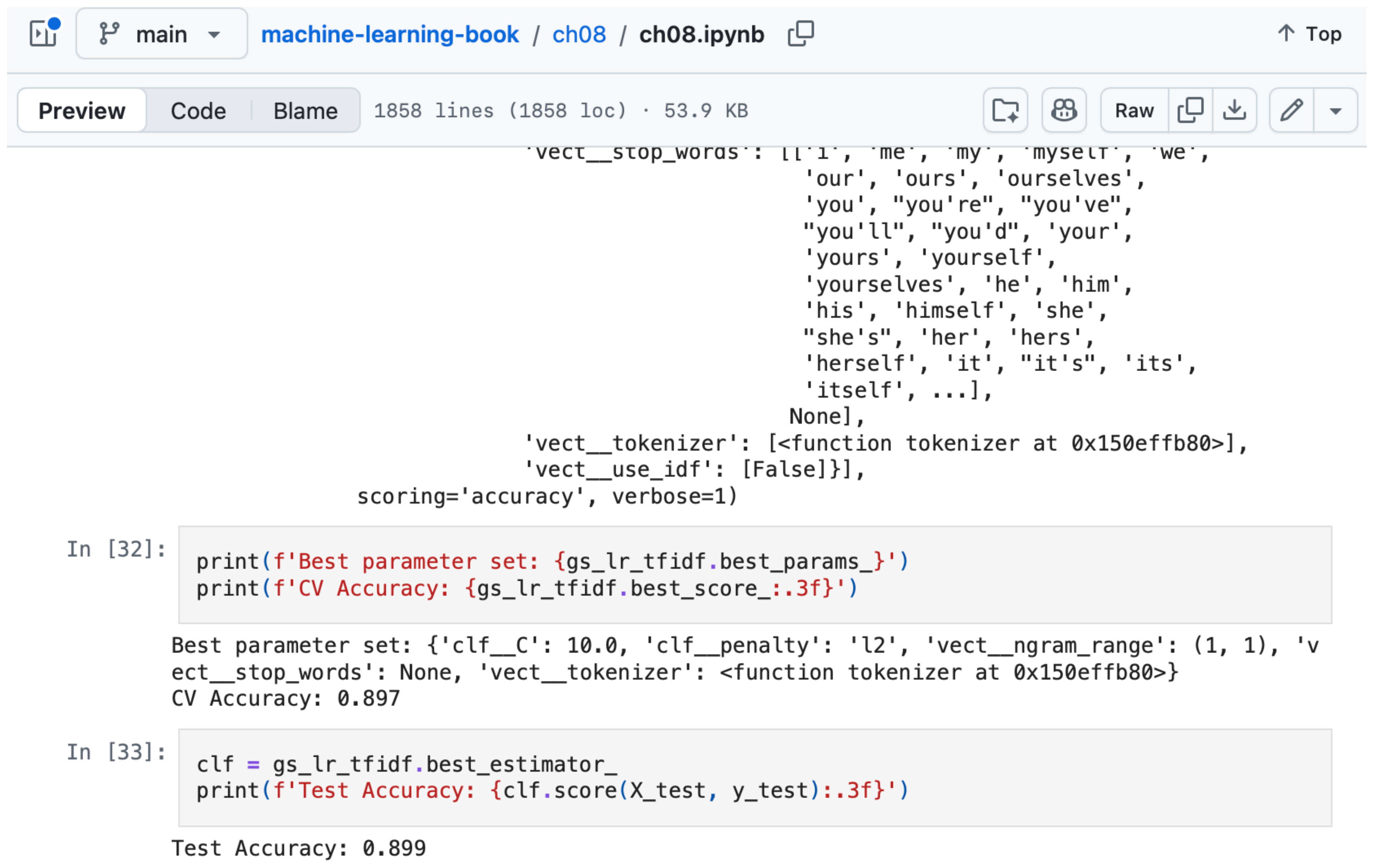
尽管存在这些缺陷,我仍然认为词袋在某些低风险应用中占有一席之地,因为它实在太便宜了;而词袋表示 + 逻辑回归仍然是我处理每一个文本分类问题的首选基线,因为它非常容易实现。
前面提到的词袋模型也可以用于(简单的)深度神经网络,比如多层感知机。但缺点依然存在:我们会丢失句子结构和词序。
不过,更复杂的神经网络架构可以避开词袋这种变通做法:卷积神经网络(CNN)和循环神经网络(RNN),它们可以将词嵌入作为输入。
首先,在把输入文本送入模型之前,我们必须将它们转换为合适的表示形式。其中一种表示是词袋(bag-of-words),另一种是词嵌入向量。区别在于,词袋向量通过统计每个词汇出现的频率来表示整段文本,而词嵌入则把单个词表示为由学习得到的数值组成的稠密向量。
词嵌入的工作原理与 LLM 中的嵌入层类似,也就是说,它们把输入 Token 转换为稠密向量。嵌入既可以在模型外部完成(例如,两种经典且流行的学习方法是 Word2Vec 和 GloVe),也可以作为神经网络架构本身的一部分,在模型训练过程中被学习和调整。
这些经典嵌入在查表时是与上下文无关的。例如,单词 “bank” 在 “river bank” 和 “bank account” 中得到的是同一个向量(你可能知道,上下文可以通过注意力等概念来处理)。
关于嵌入的更多资料,以下内容可能对你有帮助:
第 2 章:处理文本数据(这一章讲的是 LLM,但应该能让你大致理解词或 Token 的嵌入;在 LLM 的分词器中,我们把单词拆分为子词 Token;而在 Word2Vec 中,1 个单词通常就是 1 个 Token。)
理解嵌入层与线性层的区别(这份说明展示了在什么情况下嵌入向量在数学上等价于线性层和矩阵乘法。)
由于你们中的许多人可能对循环神经网络(RNN)已经很熟悉,这一节我会讲得简短一些。RNN 是自然语言处理中一种经典的常用神经网络架构,其流行变体可以追溯到 20 世纪 80 年代和 90 年代初。2017 年问世的 Transformer(其使用的注意力机制最早正是在 RNN 中引入的;简要时间线可参见我的《Understanding Large Language Models》),随后在许多 NLP 应用中逐渐取代了 RNN。
原文较长,译文为节选;译文由英文原文机器翻译,术语按行业惯例统一,可在文末展开原文核对。
查看英文原文(Language Models for Text Classification: From Bag-of-Words to Jev)
The recently released Jev AI model has been quite a cultural phenomenon in technical communities in the past 2 weeks.
While Jev aims to classify things, it’s easy to dismiss Jev as “just a classifier,” and my own view of Jev has evolved quite a bit over the past few days. In particular, my thoughts went from “classifiers used to be my bread & butter; I can easily build this myself” (more on this later) to “wow, this actually works better than I thought.”
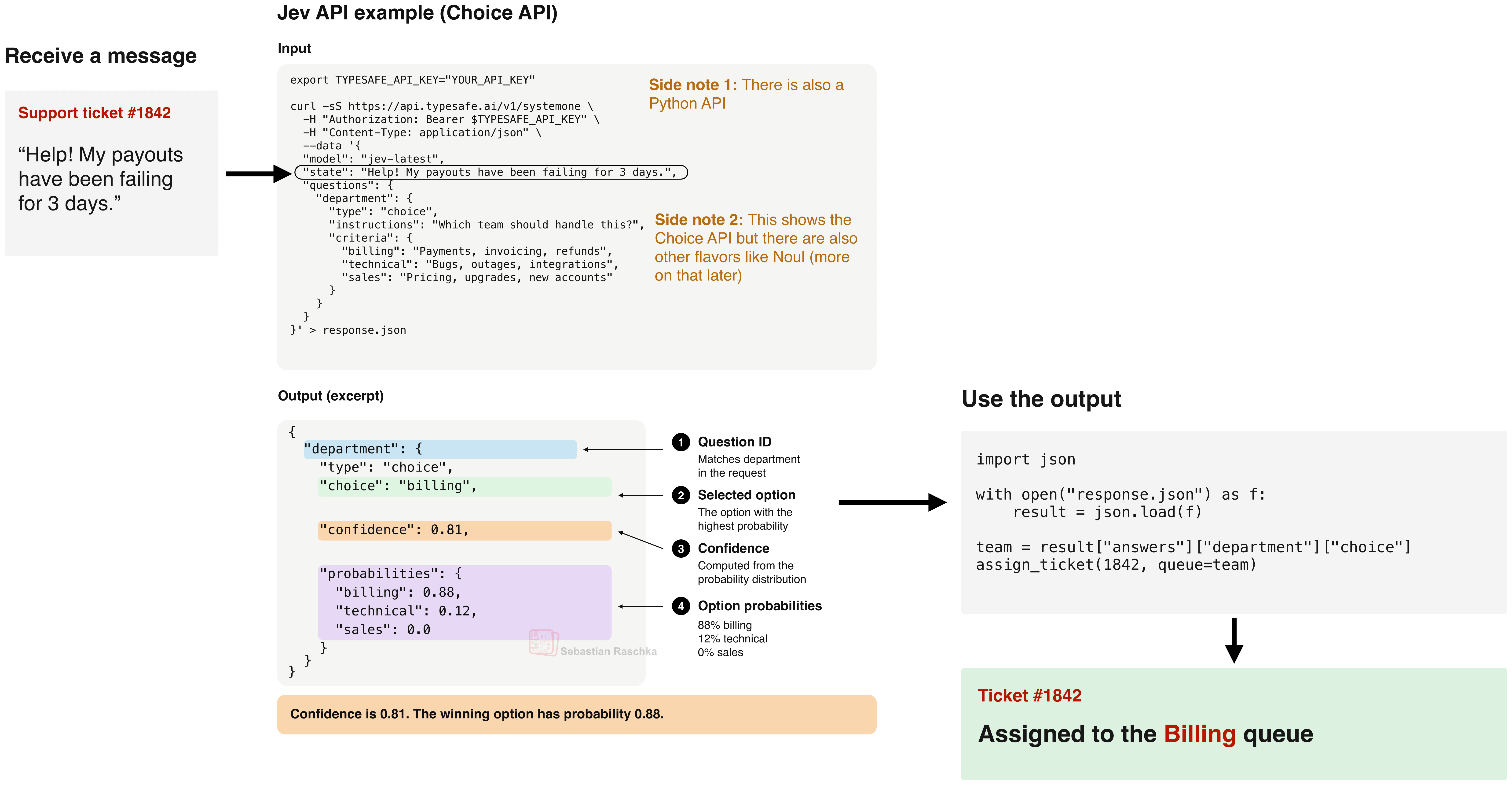
Sure, the latest state-of-the-art GPT and open-weight LLMs can do the same kinds of classification tasks as Jev, while also being capable of much more general decision-making. But Jev’s advantage is that it can handle those classification tasks much faster and more cheaply.
At the other end of the spectrum, for a narrow, well-defined problem, Jev probably won’t classify anything better, faster, or cheaper than a special-purpose classifier. But its selling point is that it is far more general than those task-specific models.
So, what is the methodology behind Jev (based on an educated guess), what can it do, and why is it so popular? I aim to answer all of these later in this article. However, I thought starting with a brief history of language models for decision-making would be a great way to begin. And it hopefully helps demystify some of the hype and show what Jev does very well (”Jev is essentially a text classifier,” but “Jev is also not ‘just’ a text classifier.”)
PS: I am not affiliated with Jev in any way. Also, I am not offered free access to Jev, and this is also not a product endorsement, just a technical article to offer some insights into the history of text classification to help you make sense of the recent hype.
Since this is a long article, I recommend reading it in your browser, where you can access the table of contents menu on the left side.
1. Language modeling and classification in the pre-transformer era
For completeness, before we put Jev in context (no pun intended), I thought it made the most sense to start chronologically. In this section, I want to take a brief tour of applied text classification via naive Bayes, logistic regression, and the more classic (deep) neural networks before transformer-based models came along.
1.1 Bag-of-words: naive Bayes, logistic regression, and XGBoost
Back in the day, when I was a grad student 15 years ago, even though recurrent neural networks already existed (more on that later), text classification was usually done with a bag-of-words representation because it was straightforward and could get good results on moderately sized datasets.
In short, we can think of the bag-of-words representation as a method that makes free-form text input of different lengths compatible with classic classifiers (naive Bayes, Logistic Regression, SVMs, Random Forest, XGBoost, to name a few), which expect a fixed-size input vector.
Popular real-world applications include anything from news article classification to email spam filtering. And yes, allegedly even Gmail’s original spam filter used a Naive Bayes model with a bag-of-words representation.
As a side note, I wrote about this approach exactly 12 years ago. It was one of the first things I shared on arXiv.
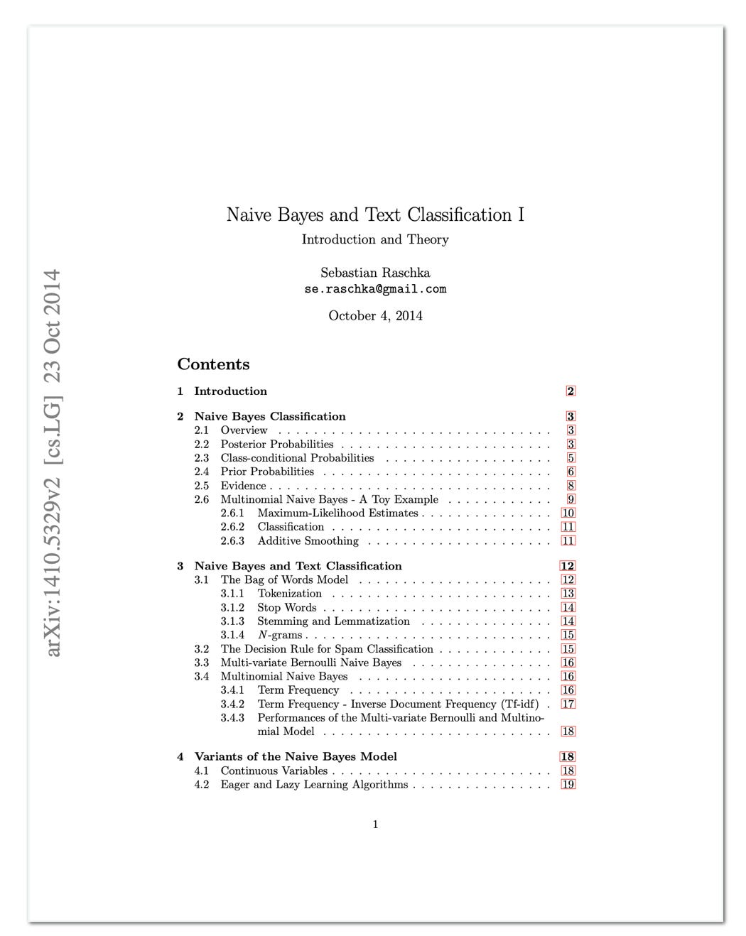
(Text classification with Naive Bayes goes back to at least 1961, where it was used to sort computer abstracts; see the Automatic Indexing: And Experimental Inquiry paper.)
So, what exactly is this bag-of-words representation? It’s a way to convert free-form texts with different lengths, e.g.,
Training example 1: “Zentropa is the most original movie I’ve seen in years. If you like unique thrillers that are influenced by film noir, then this is just the right cure for all of those Hollywood summer blockbusters clogging the theaters these days. Von Trier’s follow-ups like Breaking the Waves have gotten more acclaim, but this is really his best work.”
Training example 2: “This film is just plain horrible. John Ritter doing pratt falls, 75% of the actors delivering their lines as if they were reading them from cue cards, poor editing, horrible sound mixing”
Training example 3: “Zentropa has much in common with The Third Man, another noir-like film set among the rubble of postwar Europe.”
into a fixed-size representation for the aforementioned “classic” classifiers. (The example above is an excerpt from the popular IMDb movie review classification dataset.)
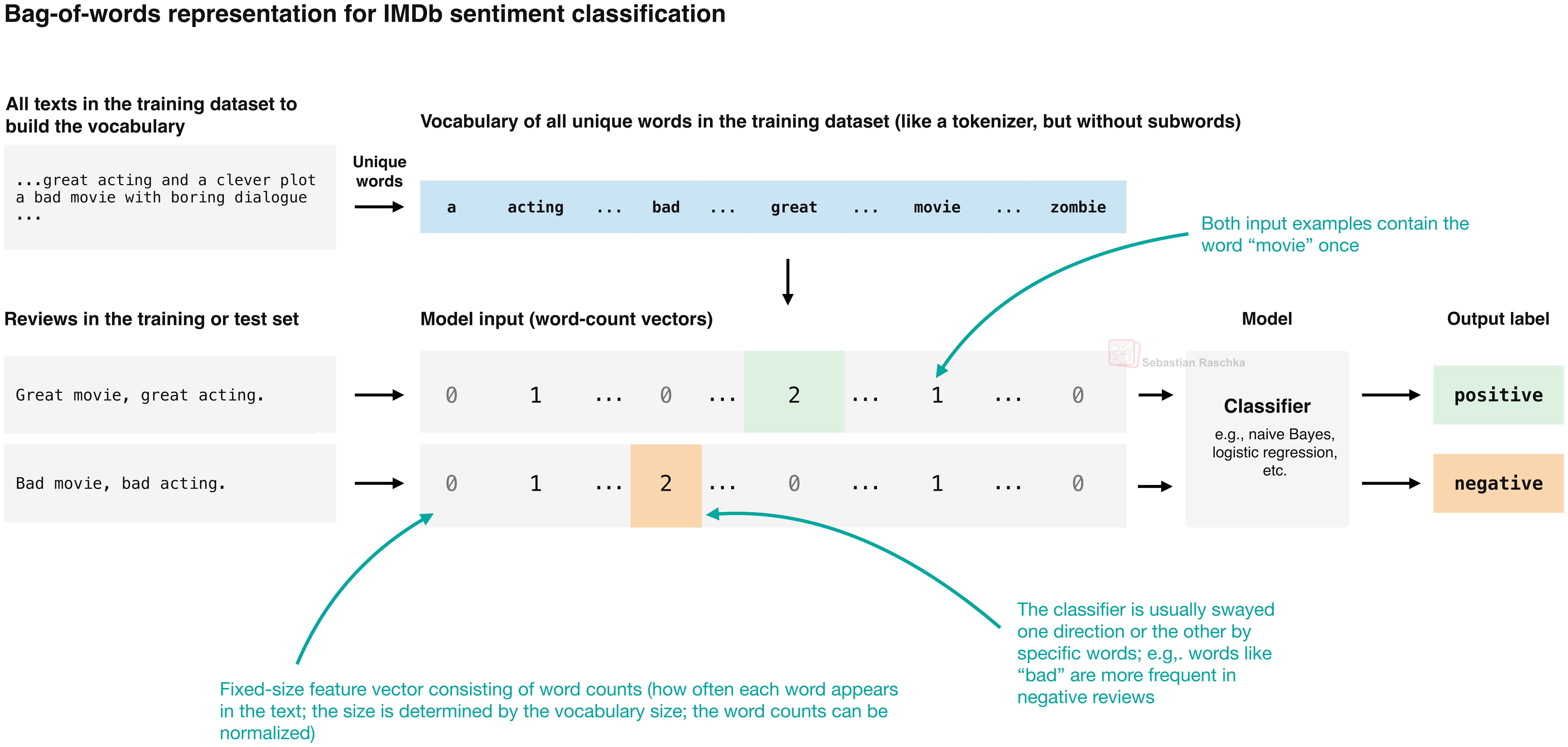
A bag-of-words model starts by building the vocabulary, which consists of all unique words in the training set (optionally, one can get rid of so-called stopwords like “a” and “the”, which are words that carry little to no semantic meaning in most contexts).
A bag-of-words representation results in these fixed-size inputs by assigning each word in a vocabulary its own position in a vector. We then count how often each word occurs in a document. For example, if we have a vocabulary of 50,000 unique words, it produces a fixed-size vector with 50,000 entries, regardless of whether the input consists of only ten words or 300k words. Note that most entries are zero because each document contains only a small subset of the vocabulary. (Instead of representing the raw counts, there are also normalization schemes like TF-IDF.)
Then, once we have these word frequency vectors, we can train a classifier on a labeled training set, such as emails labeled as spam or non-spam. For example, a logistic regression model would then learn feature weights that correlate certain words (and word counts) with particular labels. For instance, certain words might increase the predicted spam probability, and others may decrease it.
This approach is computationally cheap and can work well when particular words provide strong clues about the label. In a simple classification task such as spam classification, this is often enough to get quick, reasonably accurate results.
But one of the biggest downsides of this approach is that, because of the nature of the bag-of-words representation, it loses word order. So, for example, “the dog bites the man” and “the man bites the dog” produce identical vectors despite describing different events.
(There are some workarounds to preserve some local order by adding word pairs or longer sequences, called n-grams, as features, although this increases the vocabulary size.)
Despite the shortcomings, I still think that a bag-of-words has its place in certain low-stakes applications because it’s so cheap, and a bag-of-words representation + logistic regression remains my go-to baseline for every text classification problem, since it’s so easy to implement.
1.2 Deep neural networks for text classification
The aforementioned bag-of-words model would also work with (simple) deep neural networks, like multilayer perceptrons. But the downside still is that we would lose the sentence structure and word order.
However, more sophisticated neural network architectures avoid the bag-of-words workaround: convolutional neural networks (CNNs) and recurrent neural networks (RNNs), which can take word embeddings as input.
1.2.1 Word embeddings
First, before feeding the input texts into a model, we have to convert them into a suitable representation. One such representation is bag-of-words. Another is word embedding vectors. The difference is that a bag-of-words vector represents the entire text by counting how often each vocabulary word occurs, while a word embedding represents an individual word as a dense vector of learned numbers.
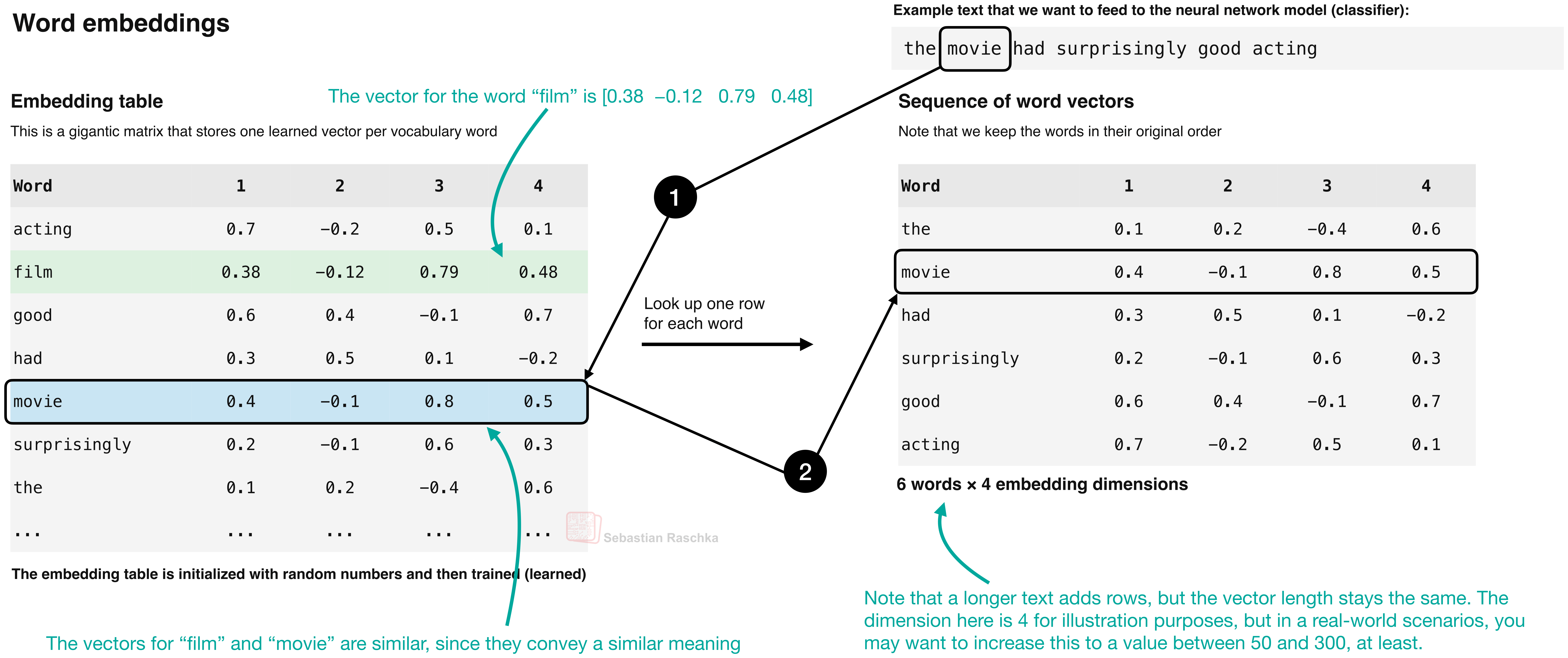
Word embeddings work similarly to embedding layers in LLMs, i.e., they convert input tokens into dense vectors. Embeddings can happen outside the model (e.g., two classic, popular methods for learning them are Word2Vec and GloVe), or the embedding layer can be part of the neural network architecture itself and be learned and tuned during model training.
These classic embeddings are context-independent at lookup time. The word “bank”, for example, gets the same vector in “river bank” and “bank account” (as you may know, context can be handled via concepts like attention).
For additional resources on embeddings, you may find the following ones helpful:
Chapter 2: Working with Text Data (this is an LLM chapter but should give you the gist of embedding words or tokens; in LLM tokenizers, we split words into subword tokens; in Word2Vec, 1 word is usually 1 token.)
Understanding the Difference Between Embedding Layers and Linear Layers (this is an illustration that shows when embedding vectors are mathematically equivalent to Linear layers and matrix multiplications.)
1.2.2 Recurrent neural networks (RNNs)
Since many of you are probably familiar with recurrent neural networks (RNNs), I will keep this section short. RNNs are a classic go-to neural network architecture for natural language processing, and popular variants go back to the 1980s and early 1990s. Transformers, which were introduced in 2017 (and using the attention mechanisms that were first introduced in RNNs; see my Understanding Large Language Models for a brief timeline), then gradually replaced them in many NLP applications.
RNNs read a sequence (like text) one word at a time. At each step, they combine the current word embedding (discussed in the previous section) with a hidden state from the previous step. We can think of the hidden state as a fixed-size vector that summarizes the text processed so far, so this makes word order matter, because rearranging the words changes the sequence of state updates.
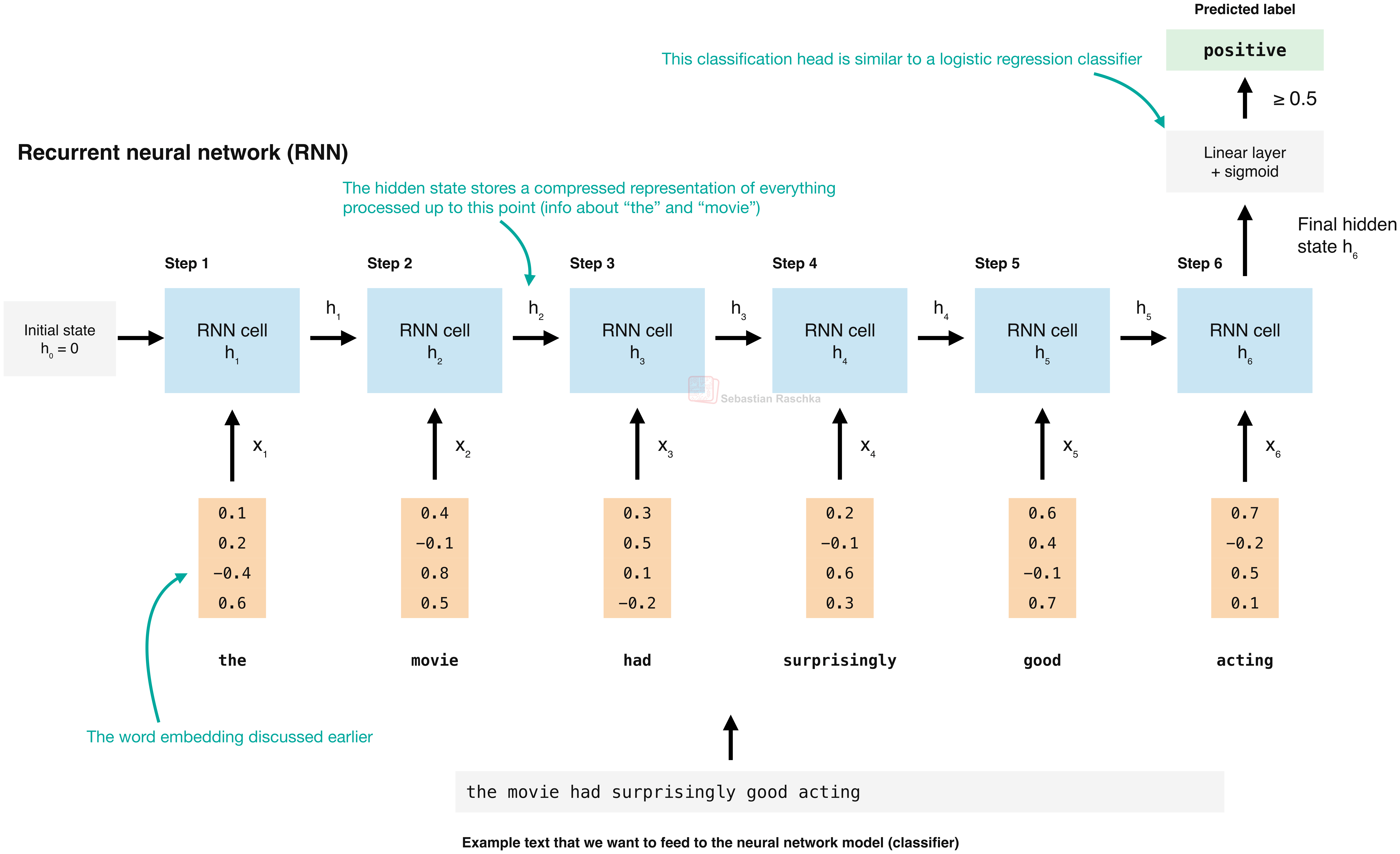
Note that the figure above shows the RNN in the unrolled representation. I.e., the RNN reuses the same layer stack for each input, hence the term “recurrent”. And since it’s “recurrent”, the input text can have an arbitrary length. The figure below illustrates the “recurrence” with the unrolled representation side by side. Note that both show the identical architecture, it’s just a different visualization.
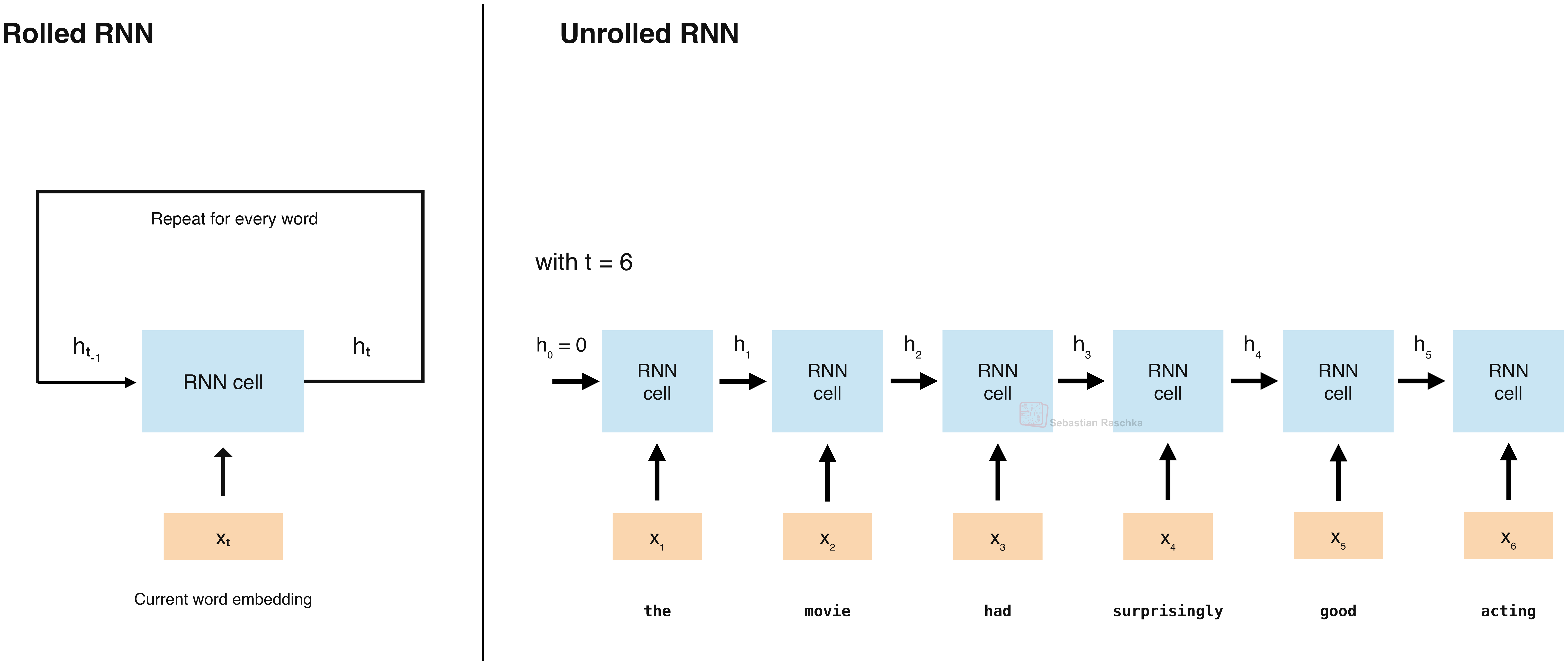
RNNs were notoriously hard to train, and there are important improvements to RNNs, like Long short-term memory (LSTM) networks, introduced in 1997, and gated recurrent units (GRUs), introduced in 2014, which use learned gates to control how information is retained and updated. (There is also the more recent xLSTM: Extended long short-term memory, introduced in 2024).
Also, state-space models are inspired by this idea of a fixed-size hidden state updated sequentially, which is cheaper than transformer attention. However, the bottleneck is still how much information the hidden state can retain, and it still has to be processed sequentially. (Fun fact: attention was first developed for RNNs before the transformer architecture came along, but it’s a story for another time; I’ve written about it in my Understanding Large Language Models article.)
The bottom line is that RNNs can be used to train text classifiers. Coming back to the IMDb movie review dataset, the bag-of-words classifier with logistic regression achieved about 89.9% accuracy (on a balanced dataset), while an LSTM RNN achieved only 85.66% accuracy. Yes, RNNs can be harder to train (stay tuned for the ULMFiT method below, which trains an RNN with much higher accuracy).
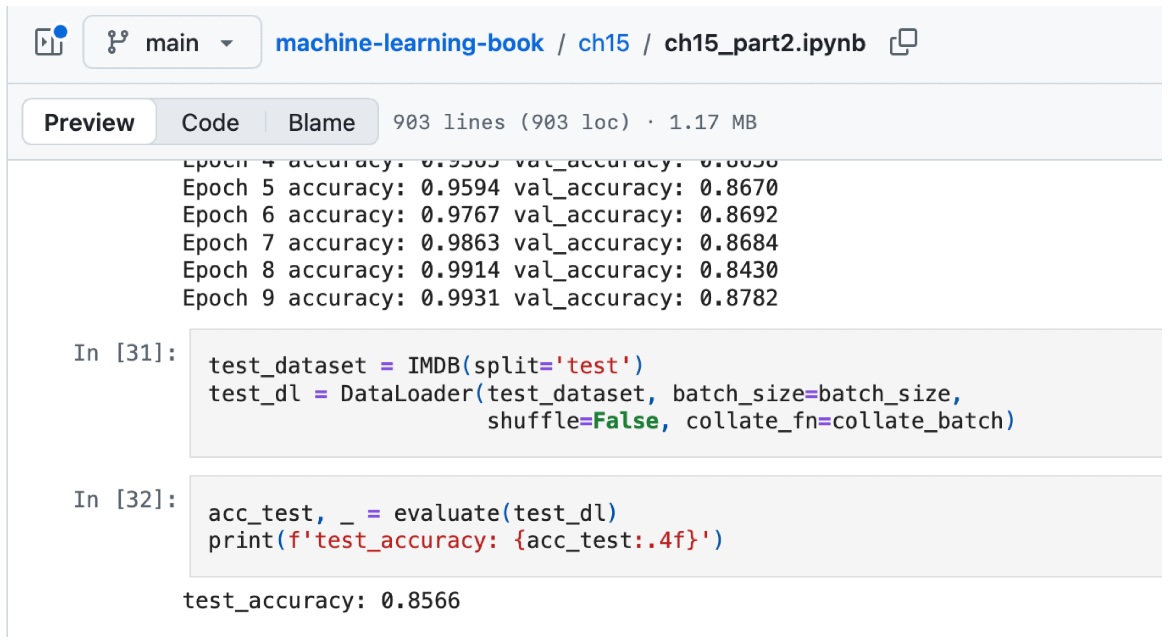
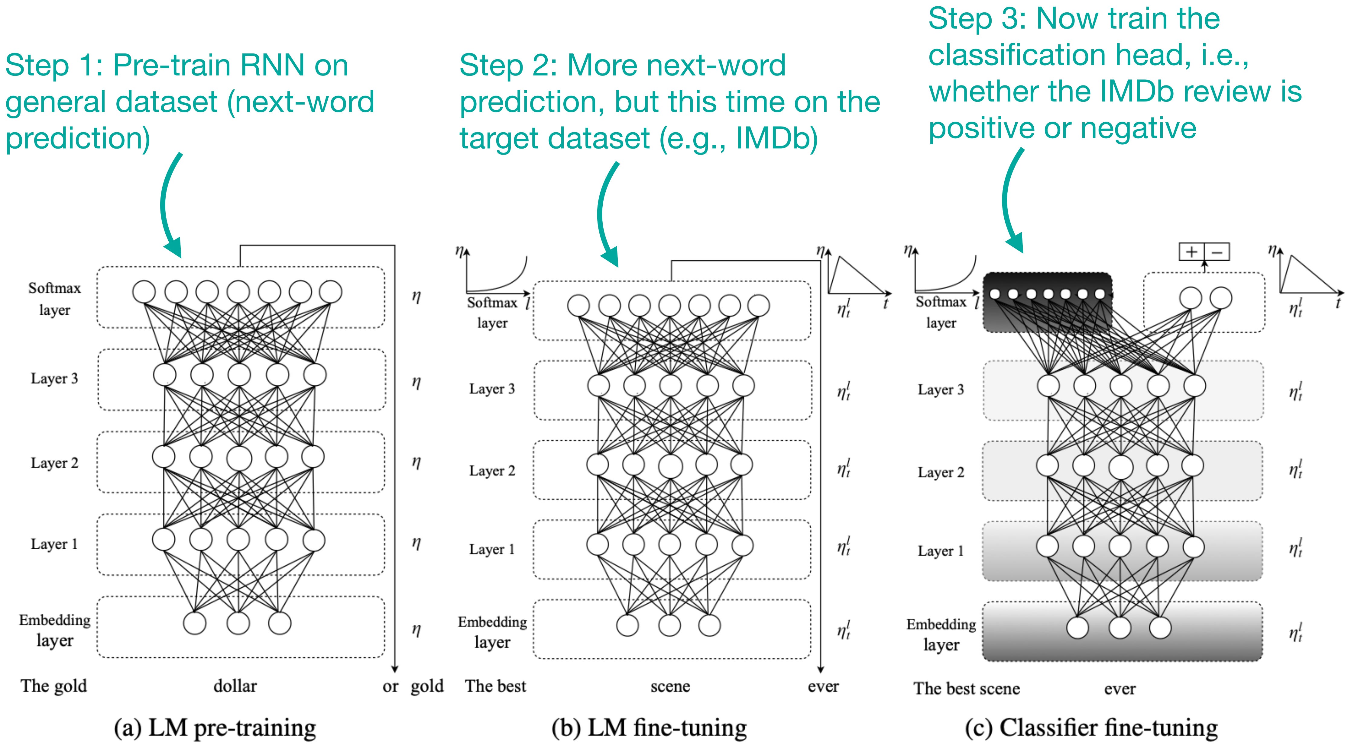
Note that this RNN was trained from scratch. A better approach is to pre-train the model on a larger dataset first, then fine-tune it on this target dataset (classically, we call this approach “transfer learning”).
In the natural language processing domain, one of the most influential papers proposing this approach is ULMFiT (2018), which achieved an impressive 95.4% test accuracy on IMDb.
1.2.3 Convolutional neural networks (CNNs)
You probably know convolutional neural networks (CNNs) from their use in computer vision. However, it is also possible, although historically less common, to use them for text.
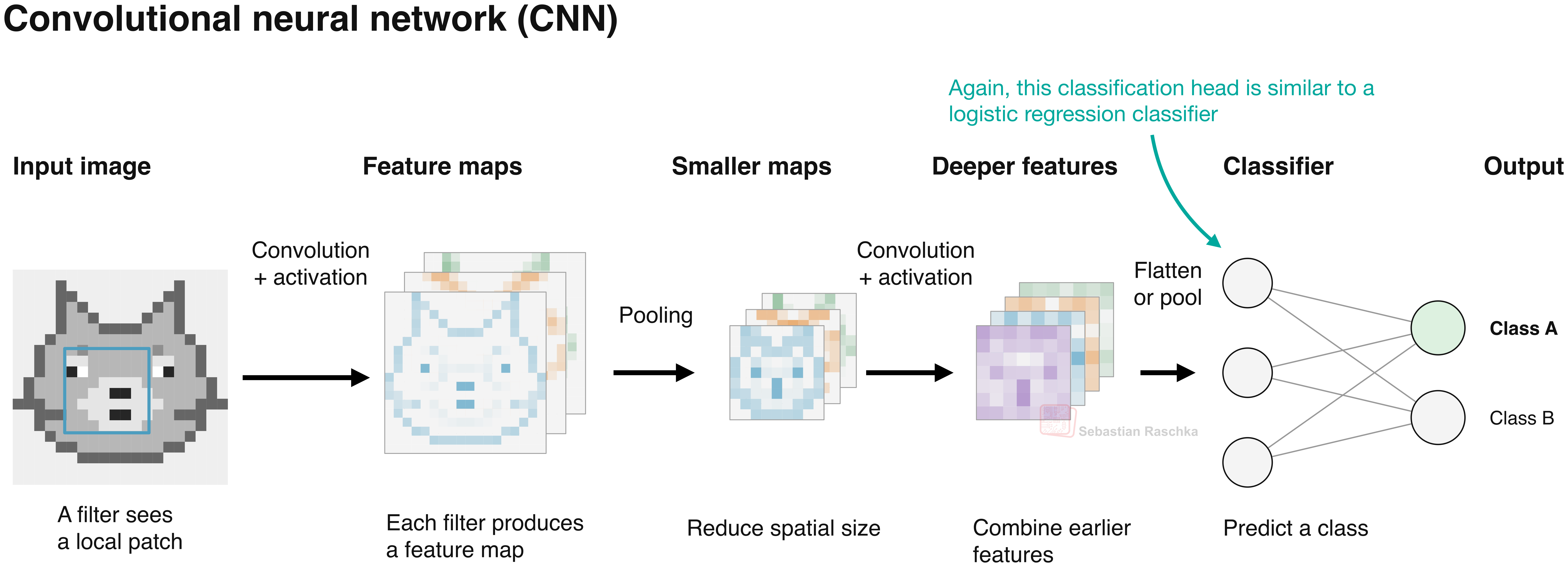
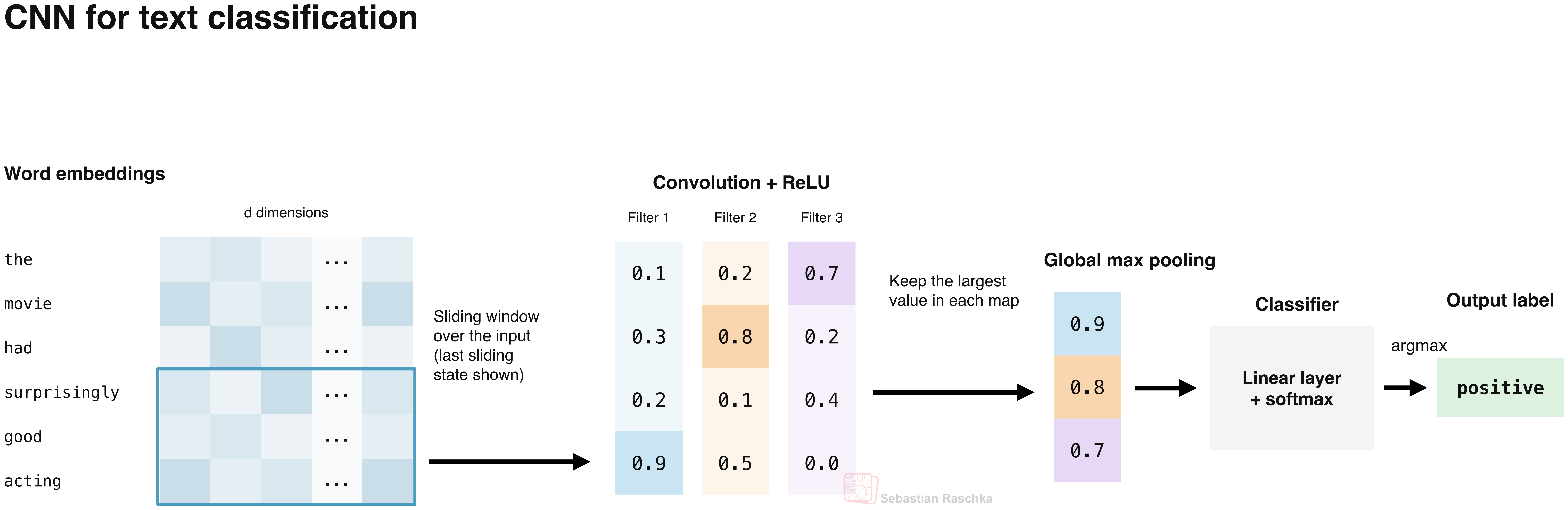
As shown in the image classification example in the figure above, CNNs apply learned filters to image patches (windows). Similarly, in the natural language domain, we can apply learned filters to windows of adjacent word embeddings.
As illustrated in the figure above, a convolutional filter with a window size of three uses the same weights for each adjacent group of three words. Then, as it slides over the inputs, it moves the filter one word at a time across “the movie had surprisingly good acting”. So, this gives four windows (ignoring padding for simplicity):
1: “the movie had”
2: “movie had surprisingly”
3: “had surprisingly good”
4: “surprisingly good acting”
So, in the last layer, before the classification head, we can either flatten or global max pool the results before connecting it to the classification head. While flattening preserves all information, it would produce differently sized vectors depending on the text input length. (E.g., if “the movie had surprisingly good acting” were longer, we would have longer feature maps.) So, to make it input-length agnostic, global max-pooling would be a better option here.
In short, we can visualize the text CNN as shown below.
Also, what’s nice is that the filter computations across positions can run in parallel, which avoids the step-by-step dependency of an RNN.
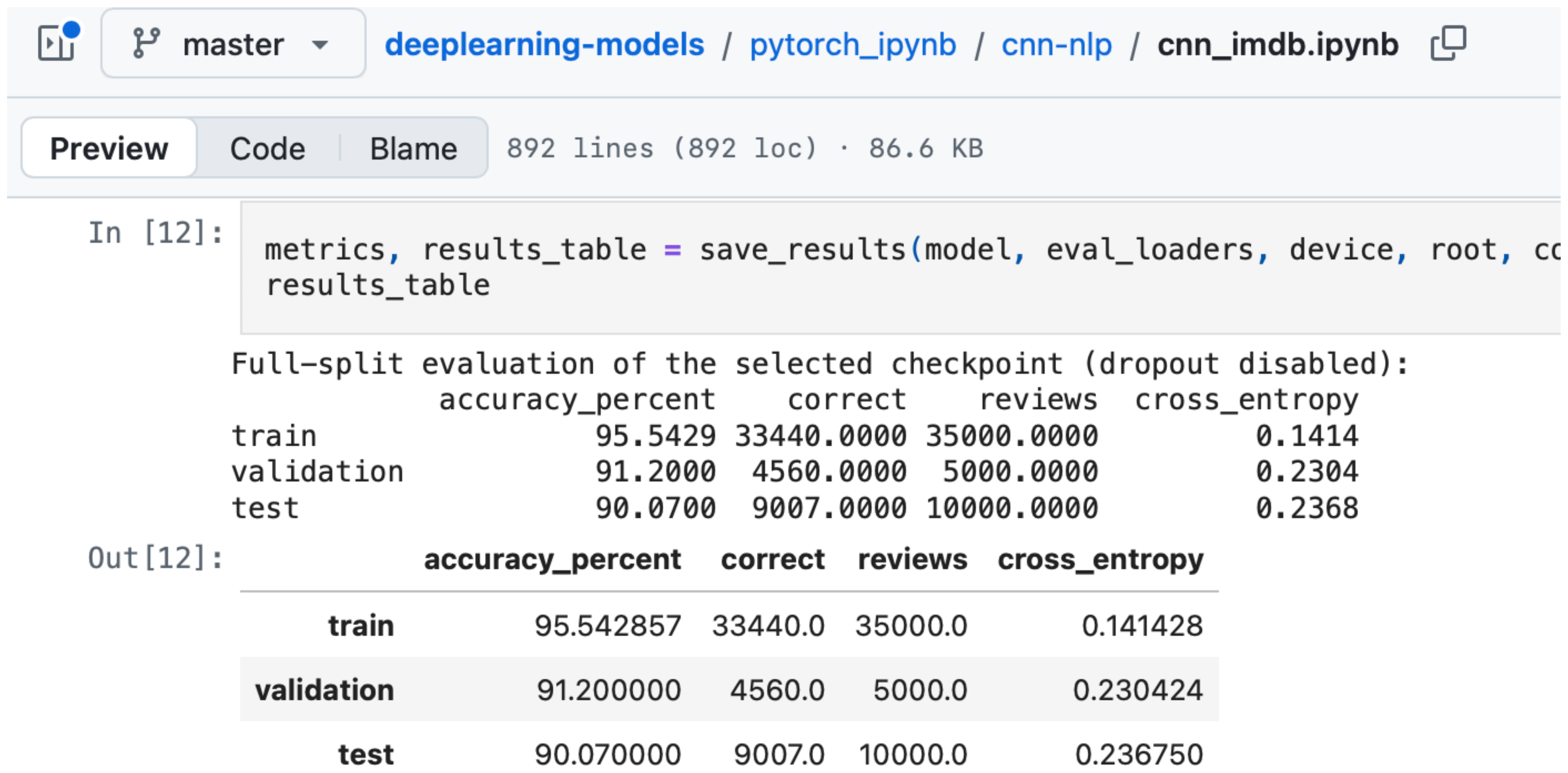
For a quick comparison, on the aforementioned IMDb dataset, my experiments show that such a CNN gets about 90.07% accuracy (but note that this is highly architecture-dependent; for example, you may know from computer vision contexts that accuracies can vary widely). (E.g., the good old AlexNet had a ~62.5% top-1 accuracy on ImageNet, and a ConvNeXt V2-H gets 88.9%.)
2. Transformers
In 2017, the original transformer architecture was introduced in the Attention Is All You Need paper. Since this topic has been covered so extensively (by me and others), I will focus on the classification-relevant aspects. But for those interested in the attention mechanism and other architecture details, please see my related articles:
The key point is that the original transformer architecture was an encoder-decoder setup used for language translation, but it can be easily adapted for text classification tasks, as I’ll illustrate in the following sections.
2.1 Encoder-style language models
I remember all too well the first years after the original transformer architecture release. They were pretty much defined by the rivalry between two different approaches:
Encoder-style models like BERT, primarily developed by Google;
Decoder-style models like GPT, primarily developed by OpenAI.
Encoder-style models were natural text classifiers, whereas GPT models could do zero- and few-shot classification as an emergent property, but their strength was more in generative tasks.
But let’s start with encoder-style models and how to fine-tune and use them to classify text.
One universal aspect of using transformers, whether encoder- or decoder-style, is that we work with models pre-trained on large text corpora, and, in addition to using them as zero- or few-shot classifiers, we can fine-tune them on the target dataset (similar to ULMFiT, as mentioned in the RNN section earlier).
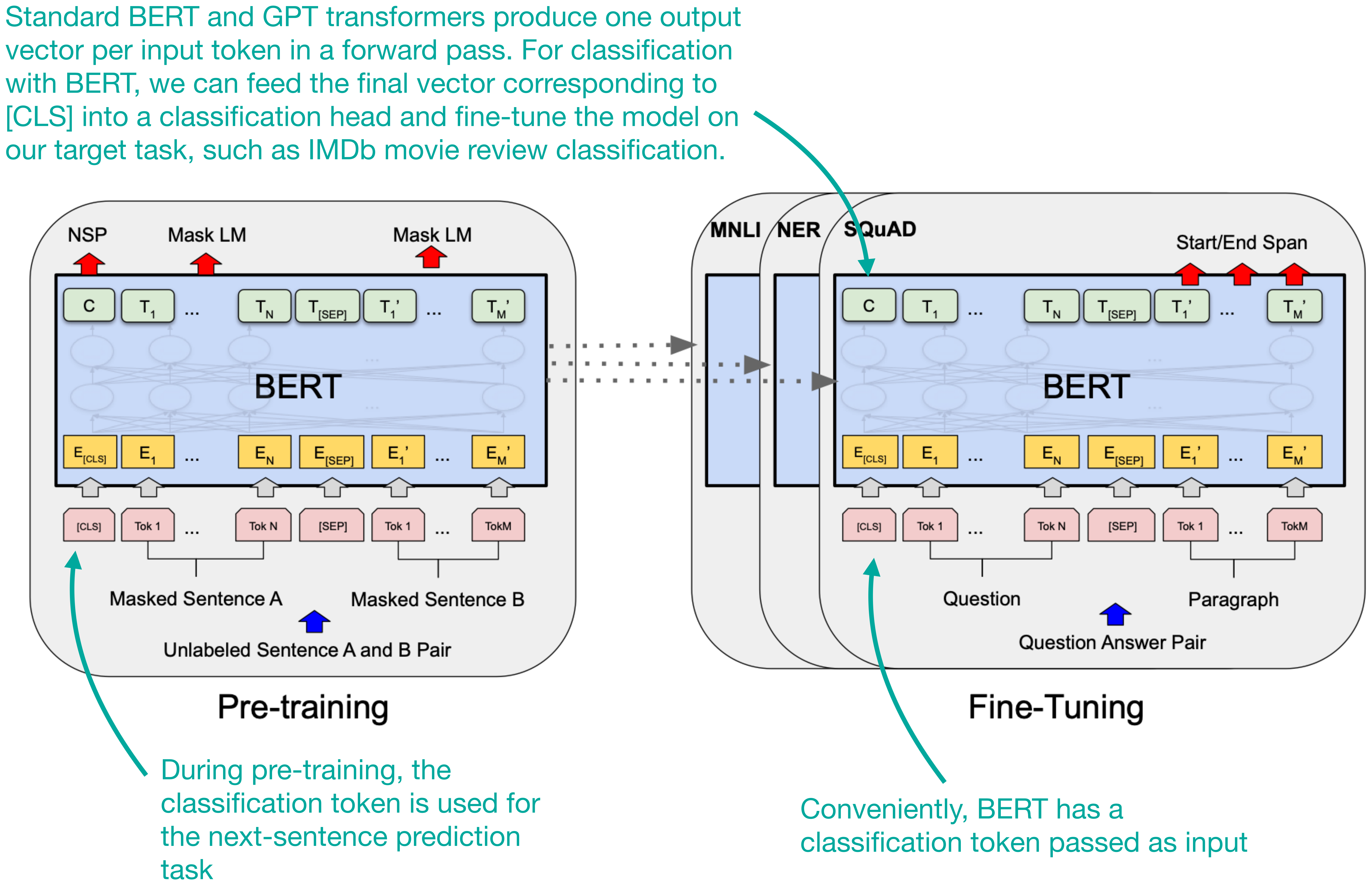
As shown in the figure excerpt from the BERT paper (2018) below, BERT-/encoder-style models have a classification token at the first position that we can conveniently fine-tune for this.
While BERT models are not nearly as popular as autoregressive GPT-style transformers, thankfully some people still update and modernize them occasionally. One recent example that is often my go-to for classification tasks is the 2024 ModernBERT model.
As shown below, on the IMDb movie reviews, ModernBERT gets approximately 95% accuracy with very little fine-tuning effort.
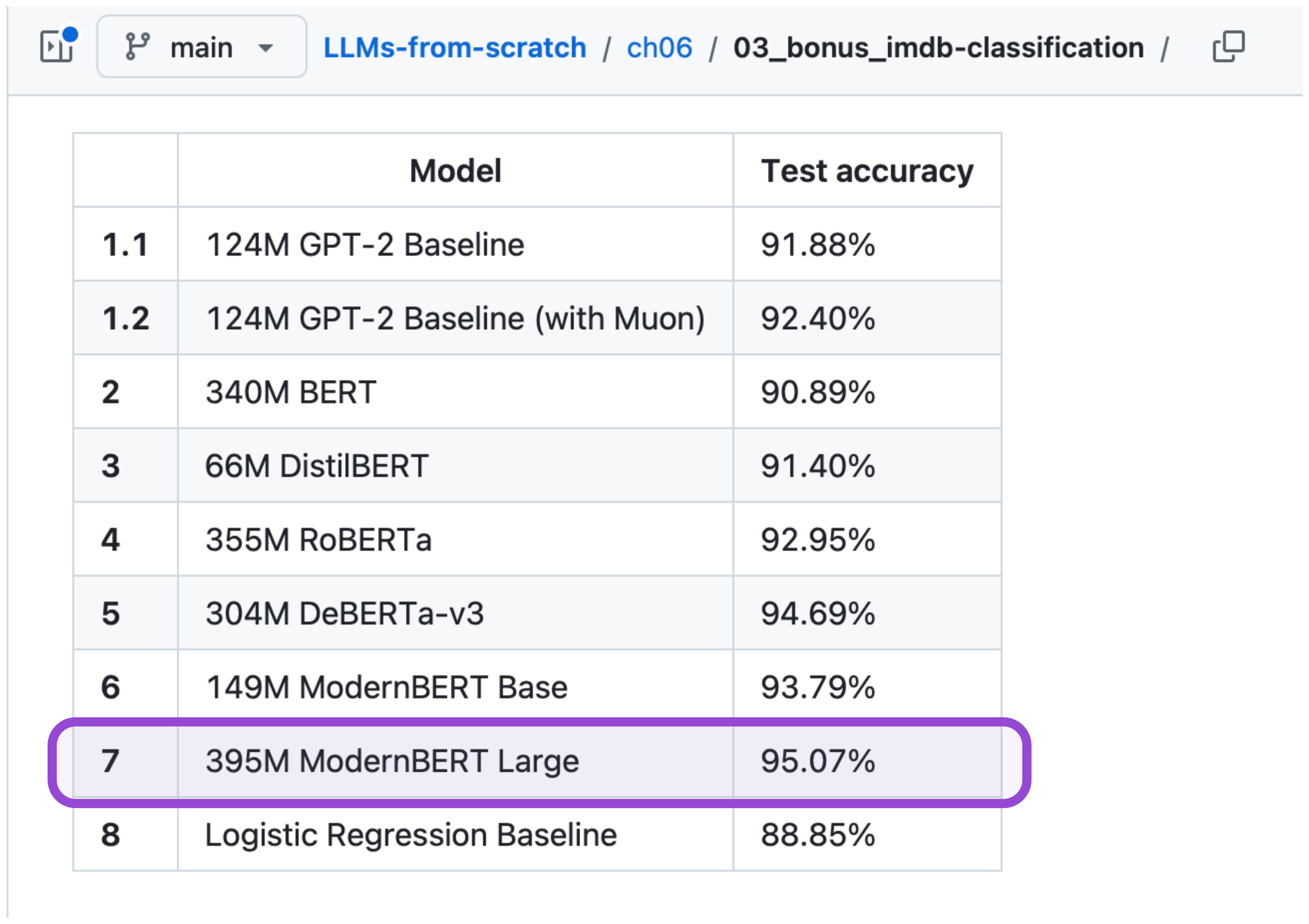
2.2 Decoder-style LLMs
LLMs like GPT are decoder-style, autoregressive transformers that are the center of all attention (no pun intended) for generating text and code.
However, as I explained in chapter 6 of my Build A Large Language Model (From Scratch) book, as a gentle introduction to fine-tuning (before covering instruction fine-tuning), we can also repurpose these for text classification.
Sure, we can also prompt an LLM directly, as shown in the screenshot below.
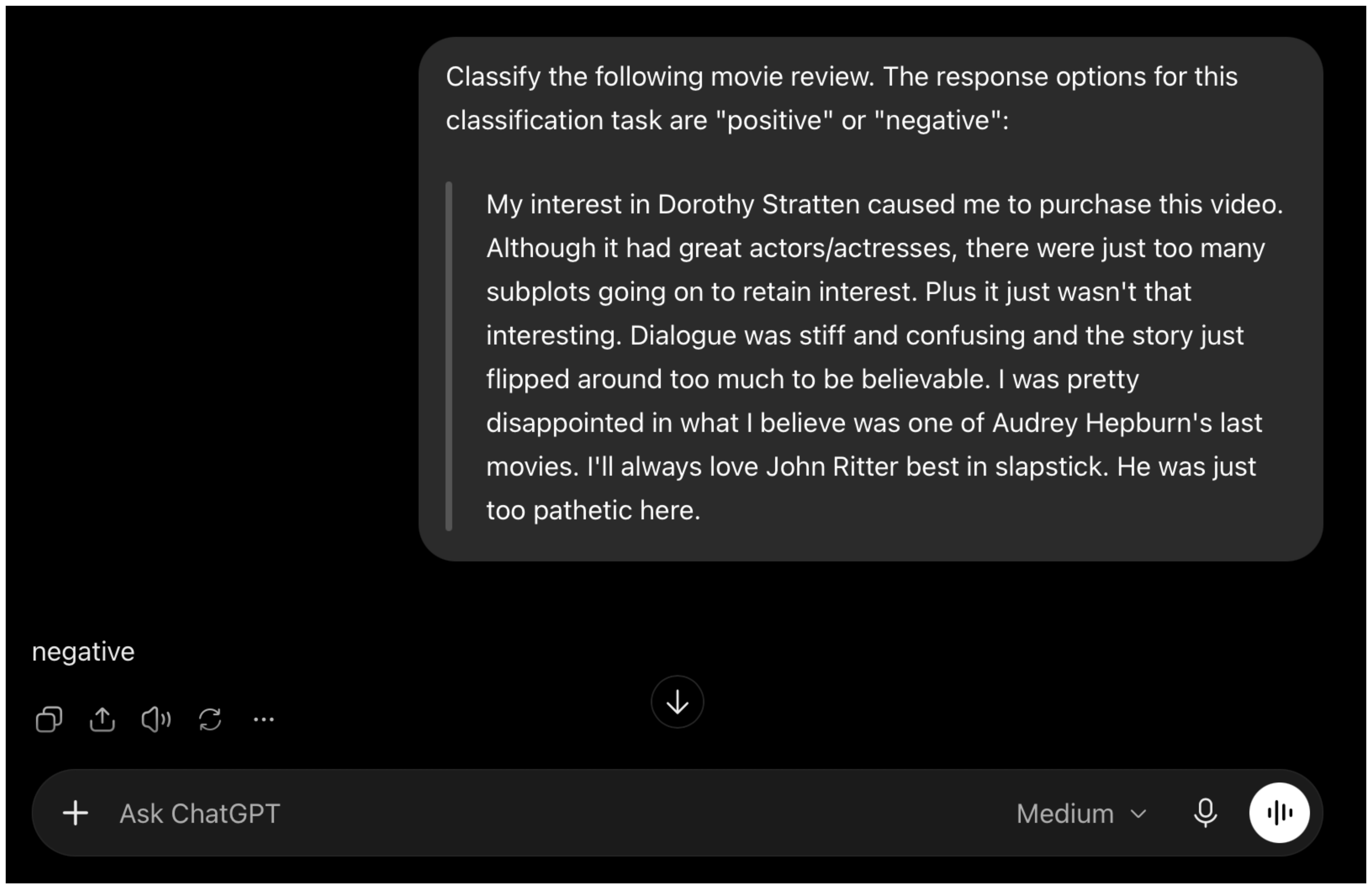
However, if we want structured outputs and we have
正文保留英文原文,标题与摘要由机器翻译。
原文发布于 Sebastian Raschka(Language Models for Text Classification: From Bag-of-Words to Jev),标题、摘要与正文由机器翻译,术语按行业惯例统一,未经人工逐句校订。